Representation learning

Erik Ylipää (erik.ylipaa@liu.se)

NBIS

08-May-2026

Outline

• Representation learning
• Supervised representation learning
• Contrastive learning
• Self-supervised learning
• Multimodal Learning
• Summary

Representation learning

AI subfields

Deep learning is a subset of machine learning. But what makes deep learning special?

AI subfields: Representation Learning

Data representation is crucial for learning

The way we represent data has a huge impact on how easy a problem is to solve. This toy example illustrates that in a cartesian representation, the classes are hard to easily separate, while in a polar representation they become linearly separable.

Shallow representations – Principal Component Analysis (PCA)

Neural Networks learn representations from data

The fundamental idea of neural networks and deep learning is that we learn to map the input data into new representations which are more useful for the downstreams layers (helping them reduce the loss). Each layer learns a transformation of the data into a new space, and the final layers typically use a linear model (e.g. linear or multinomial logistic regression) to make predictions. In deep learning, we often talk about learning signals, the signal which drives the learning of representations. By crafting the network in different ways, and adjusting what the loss function penalizes we can drive the learning of different representations. For example, in supervised learning, the learning signal is the error between the predicted labels and the true labels.

Transfer learning

While there are many advantages to deep representation learning, one powerful consequence is that we can transfer the learned representations to new tasks. For example, a model trained on ImageNet learns general features that can be useful for many other vision tasks, even if the new task has limited data. This is known as transfer learning and is a key reason why deep learning has been so successful in practice.

Supervised representation learning

The classification head

https://www.mathworks.com/discovery/convolutional-neural-network.html

The classification head typically has a fully connected layer followed by a softmax. The fully connected layer is what we’ll look at here.

What is the core mechanism of neural networks?

\vec{y} = \operatorname{softmax}(W \vec{x} + \vec{\beta})

\Leftrightarrow

\vec{y} = \operatorname{softmax}( \begin{bmatrix} \vec{w}_1^\top \\ \vdots \\ \vec{w}_n^\top \end{bmatrix} \vec{x} + \vec{\beta})

A matrix multiplication can be though of as a list of separate dot products.

The core mechanism of neural networks is the dot product

Properties of the dot product

\vec{a} \cdot \vec{b} = |\vec{a}||\vec{b}| \cos\theta

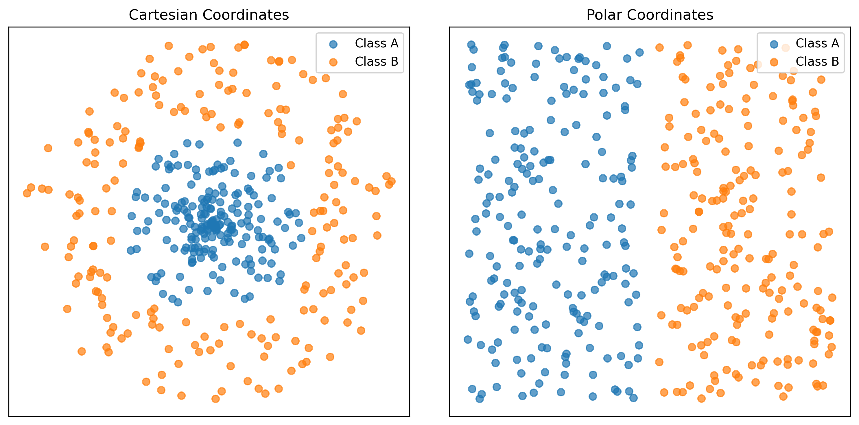
• Dot product is directly connected to the angle (alignment) between vectors
• Neural Network learns by aligning vectors

The cosine similarity is essentially the dot product of unit vectors. When two representations are identical in direction, cosine similarity = 1; orthogonal = 0; opposite = −1.

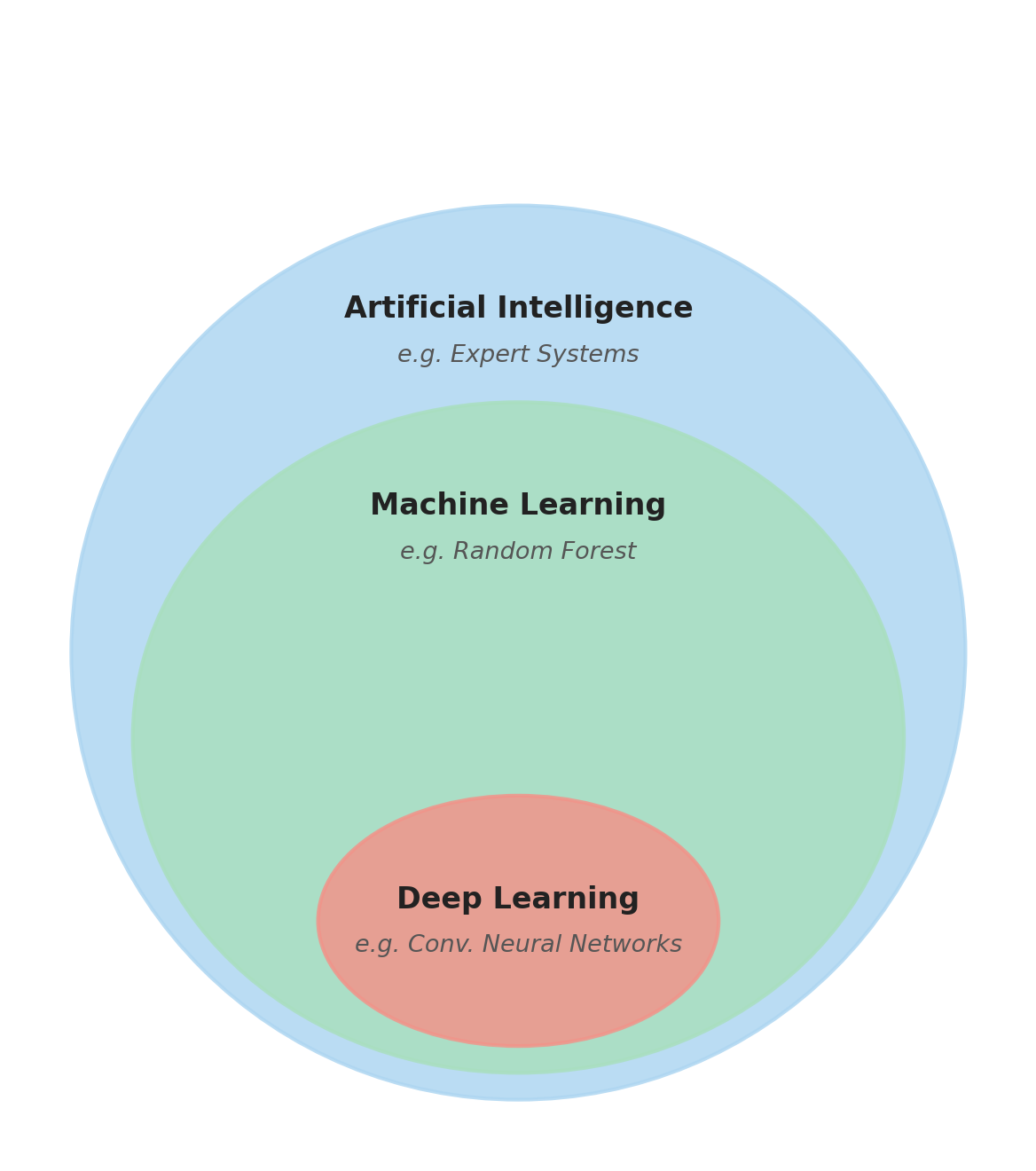
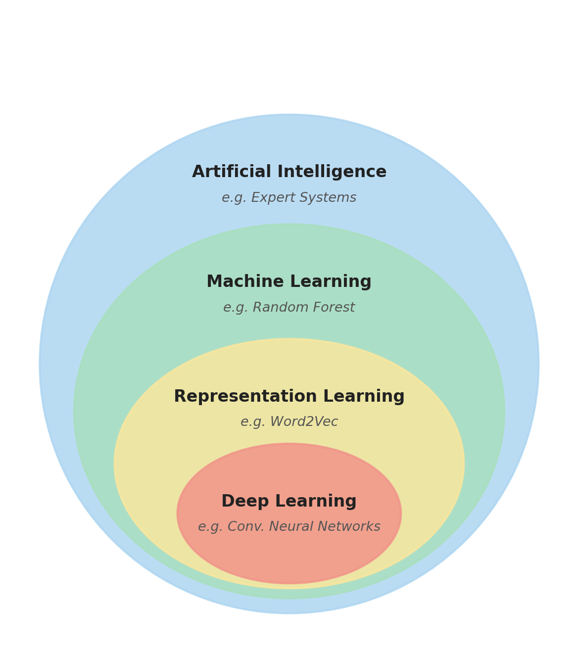
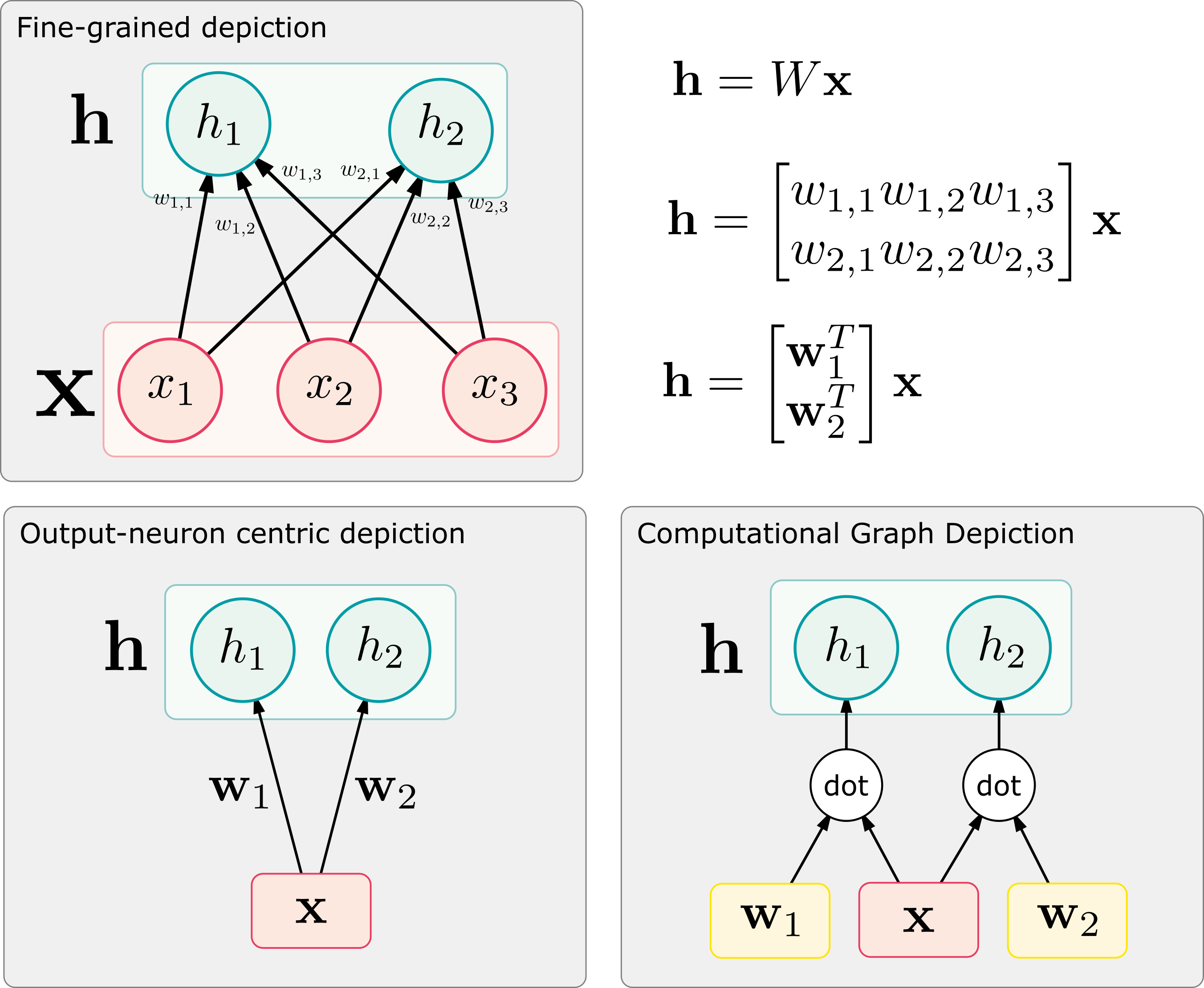
Graphical representations of neural networks

Different graphical representations of neural networks

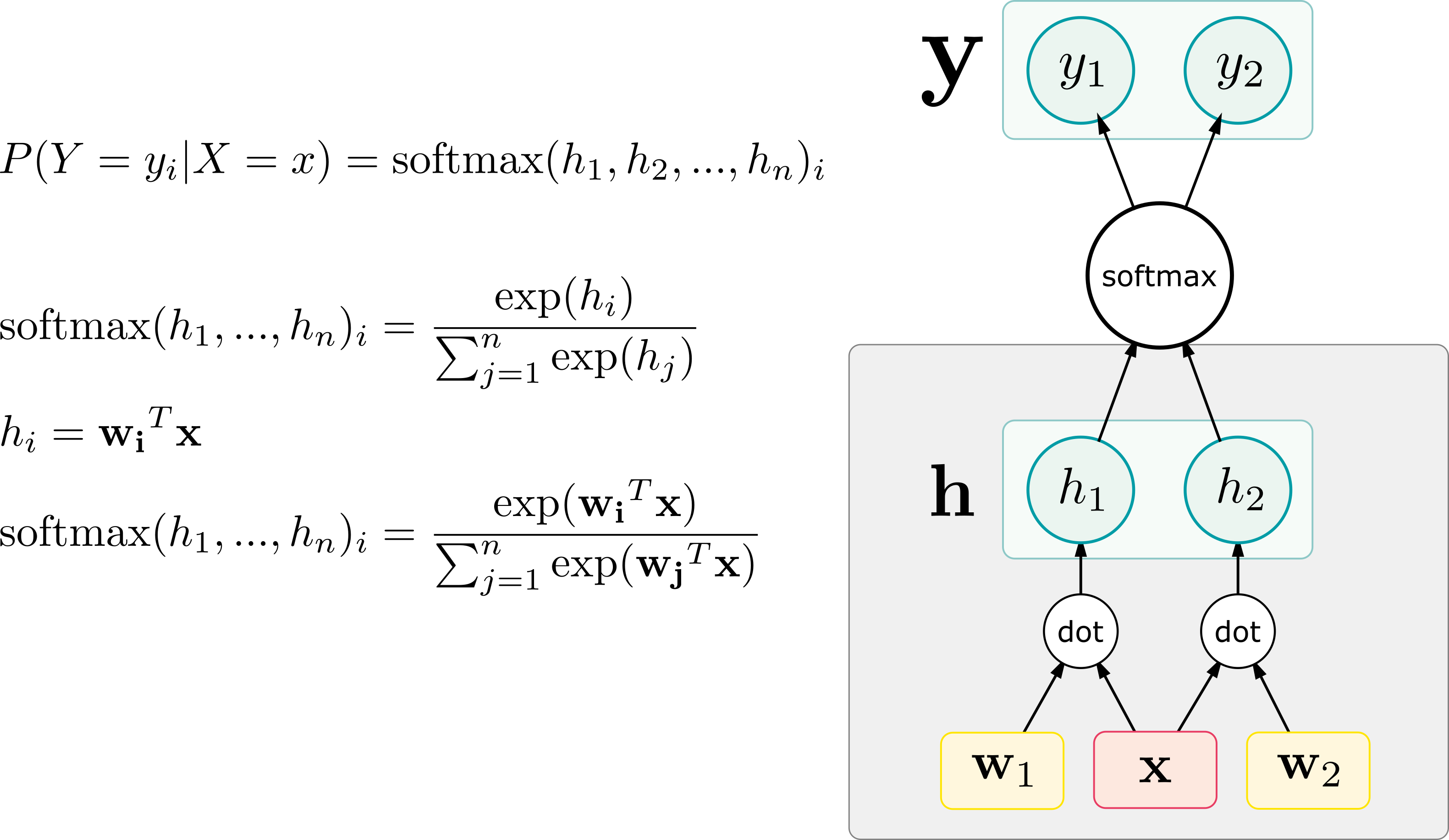
Graphically representing softmax

Computational graph view of softmax

Graphically representing softmax

Computational graph view of softmax

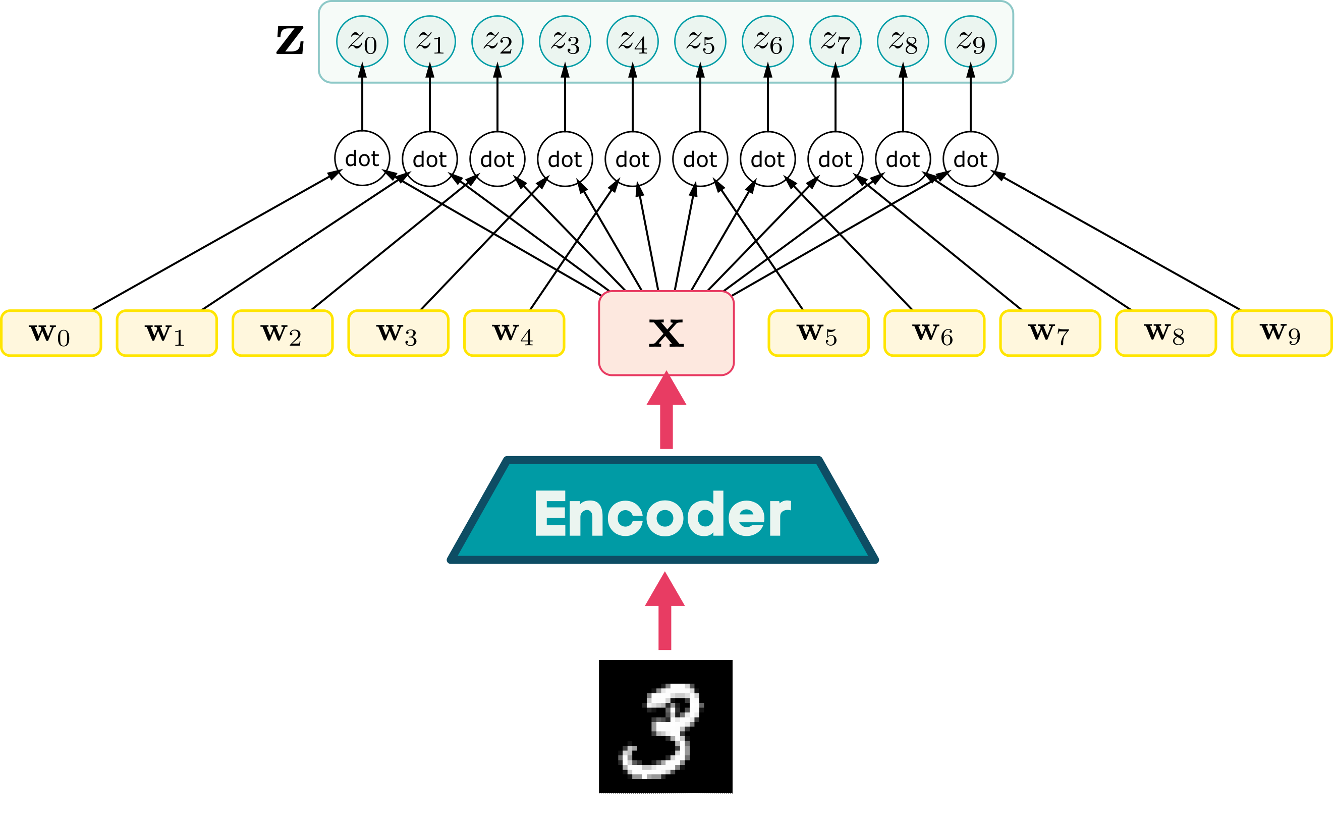
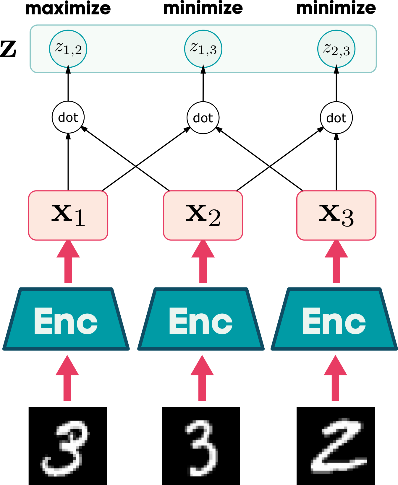
MNIST example

Softmax angle alignment

Computational graph view of softmax

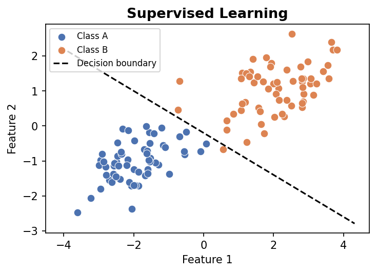
Contrastive learning

Using computed “softmax” weights

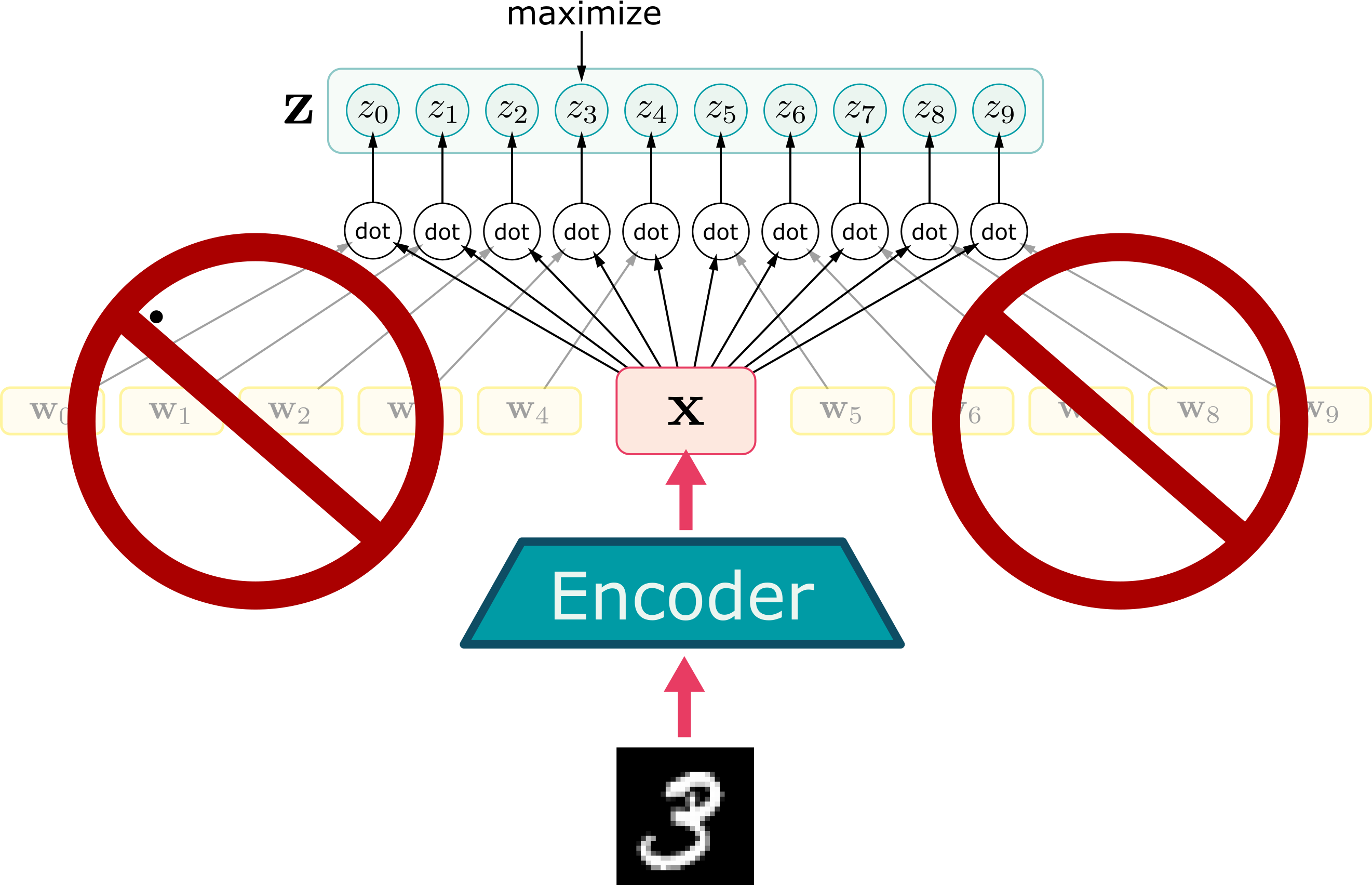
No fixed “class” vectors

Embeddings of other examples act as the “class” vectors

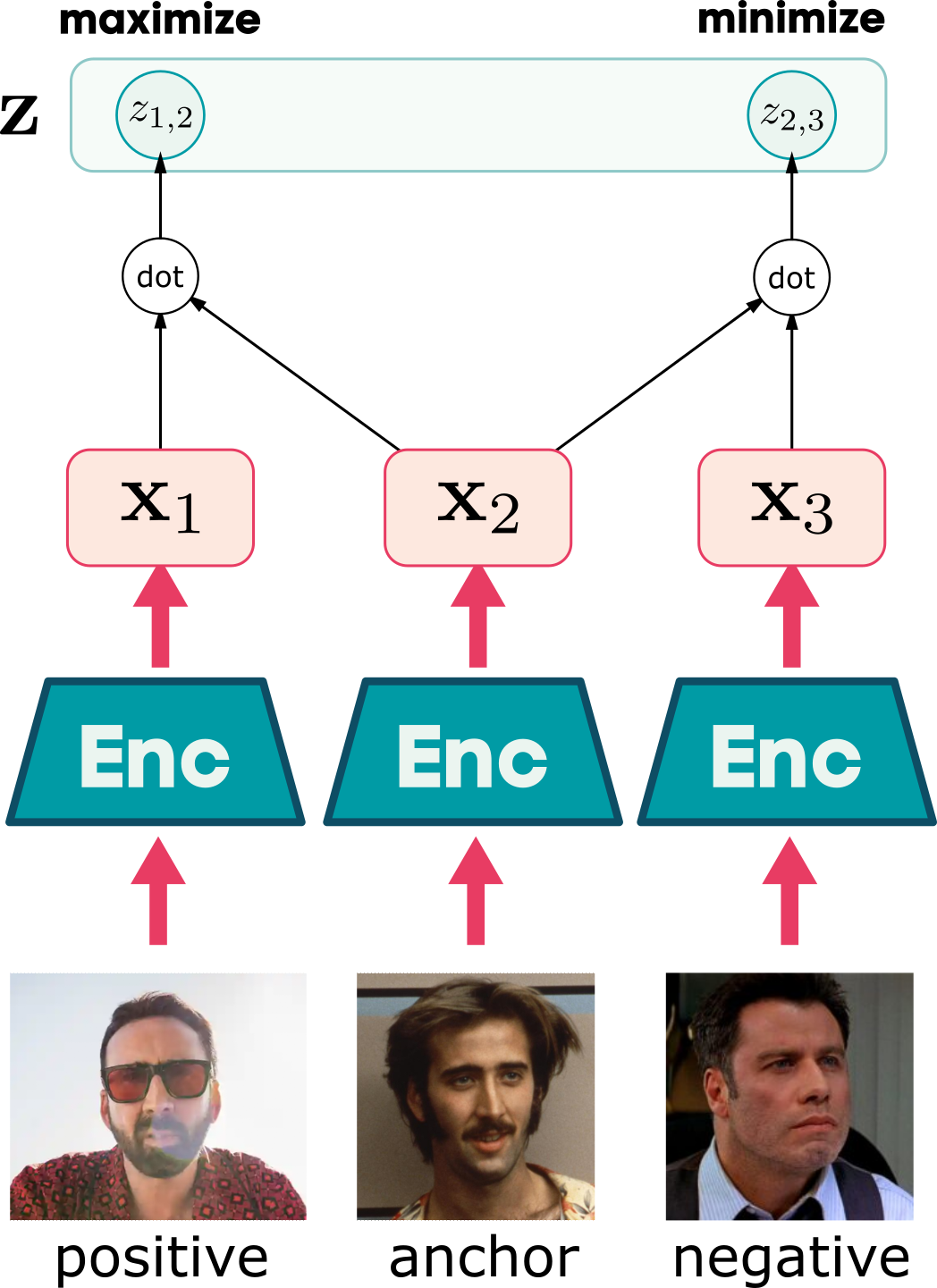
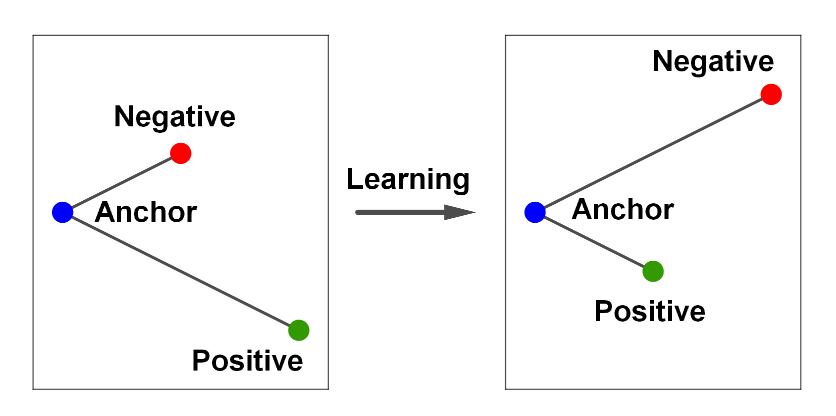
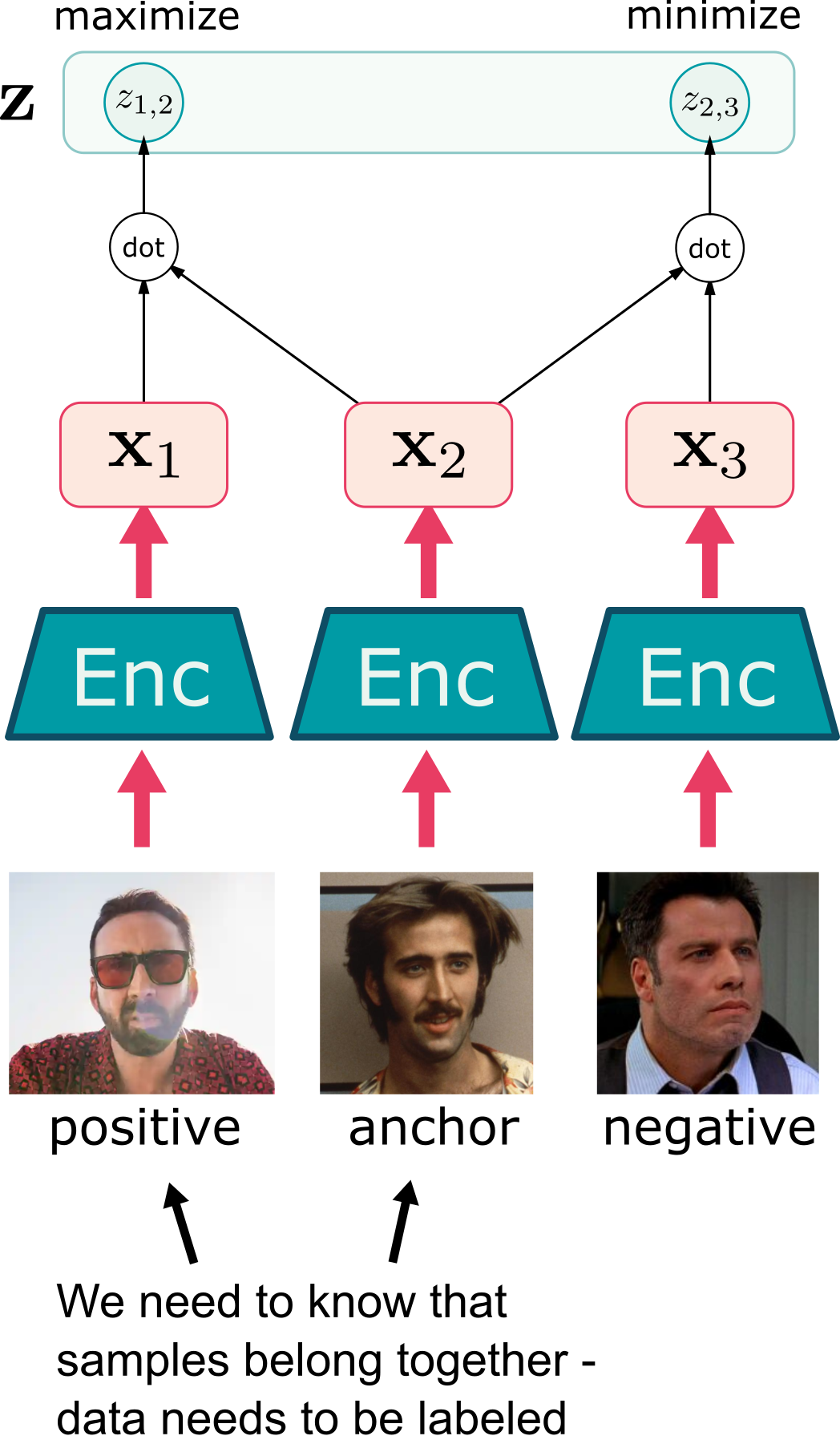
Contrastive learning - triplet loss

By Krishnachandranvn - Own work, CC BY-SA 4.0, https://commons.wikimedia.org/w/index.php?curid=138534332

The kind of loss used here was used a lot in face identification and referred to as triplet loss, three different data points are used where two consists of a positive pair which we try to align (maximize the dot product), while the negative pair should have maximum dot product. The idea was that we want to learn a metric over our data points which is semantic. Things which are close together are semantically similar (images of the same person).

What would happen if we didn’t have any negative pairs?

Triplet loss — the formula

Each training step takes three L2-normalised embeddings — an anchor x_a, a positive x_p (same class), and a negative x_n (different class) — and asks the model to align the anchor with the positive more than with the negative:

\mathcal{L}_{\text{triplet}} = \max\!\Bigl(0,\; \underbrace{-\, x_a \cdot x_p}_{\text{attract positive}} + \underbrace{x_a \cdot x_n}_{\text{repel negative}} + \underbrace{m}_{\text{margin}}\Bigr)

• x_a \cdot x_p — cosine similarity to the positive; we want this high (close to 1), so the term -x_a \cdot x_p contributes negatively — the loss decreases as the positive aligns.
• x_a \cdot x_n — cosine similarity to the negative; we want this low (close to −1), so this term pushes the loss up if the negative is too close.
• m > 0 (margin) — enforces a minimum separation: x_a \cdot x_p - x_a \cdot x_n \geq m. Without it, collapsing all embeddings to one point satisfies both terms trivially.
• \max(0, \cdot) (hinge) — the loss is exactly zero once the margin is satisfied; gradients vanish on already-correct triples.

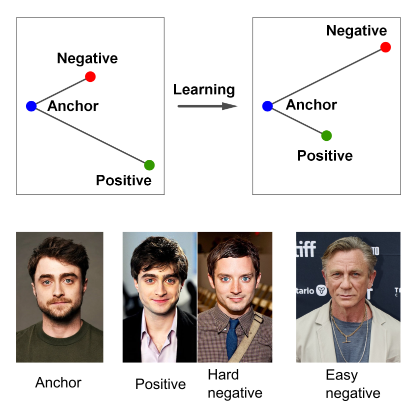
Negative samples

Even when the formula is satisfied on average, the model can stagnate if the chosen negatives are too easy:

\mathcal{L}_{\text{triplet}} = \max\!\Bigl(0,\; s^- - s^+ + m\Bigr), \qquad s^+ = x_a \cdot x_p,\quad s^- = x_a \cdot x_n

Triplet loss comparisons

Situation	s^- - s^+ + m	Gradient
Easy negative: s^+ already \gg s^- + m	< 0	Zero — no update
Semi-hard negative: s^- < s^+ but s^+ - s^- < m	(0, m)	Small corrective push
Hard negative: s^- > s^+	> m	Large corrective update

Most randomly sampled negatives are easy; the model therefore needs a hard-negative mining strategy to find informative triples. This adds overhead to the training since we need to introduce a clustering phase which recalculates the neighborhoods at regular intervals.

The setup learns more from hard negatives

While the idea of triplet loss and non-parametric softmax is to remove the fixed class vectors, the problem is still supervised in the sense that we need to know what data points we should bring together and which ones we should pull apart. Empirically it’s not necessarily better to use contrastive loss like this

Supervised Contrastive (SupCon) loss

Instead of one positive and one negative per anchor, the SupCon loss uses all same-class examples in the batch (i \in I) as positives and all other examples as negatives simultaneously:

\mathcal{L}_{\text{SupCon}} = \sum_{i \in I} \frac{-1}{|P(i)|} \sum_{p \in P(i)} \log \underbrace{\frac{\exp\!\bigl(x_i \cdot x_p \;/\; \tau\bigr)}{\displaystyle\sum_{k \in A(i)} \exp\!\bigl(x_i \cdot x_k \;/\; \tau\bigr)}}_{\text{softmax probability of drawing positive } p}

Symbol	Meaning
x_i	L2-normalised embedding of anchor i
P(i)	All same-class examples in the batch, excluding i itself
A(i)	All other examples in the batch, excluding i
\tau	Temperature: lower \tau sharpens the distribution, penalising near-miss negatives more harshly
\tfrac{1}{\lvert P(i)\rvert}	Average over positives — more positives per anchor gives a more stable gradient signal

• The numerator rewards high cosine similarity between anchor and each positive.
• The denominator normalizes against every other pair, so the model cannot escape by inflating all dot products equally.
• The \max(0,\cdot) hinge is gone; the softmax denominator acts as a continuous repulsion against all negatives at once, reducing the need for hard-negative mining.

Khosla, Prannay, et al. “Supervised contrastive learning.” Advances in neural information processing systems 33 (2020): 18661-18673.

Contrastive learning example

Why negative examples - Representation collapse

Why contrastive learning

• No need to decide on number of classes beforehand
• We only need to know that some inputs are associated and some are not
• By choosing what examples are negative vs. positive, we get a flexible framework for steering learning

Supervised contrastive learning

Contrastive learning like we’ve seen here still needs labeled data, just like regular supervised learning

Most problems we want to solve are supervised, we want to learn a mapping from inputs to outputs. However, supervised learning relies on labeled data, which can be expensive and time-consuming to obtain. In contrast, unsupervised learning can discover structure in data without labels, but is often more useful for exploratory analysis than for solving specific tasks.

The practical meaning of supervised learning – labeling

The main challenge in supervised learning is obtaining labeled data, which can be expensive and time-consuming to collect and annotate. For certain problems, such as rare disease, we are fundamentally limited in how much labeled data we can get. This motivates the need for methods that can learn from unlabeled data.

Self-supervised learning

Self-supervised learning

What if we can use the data itself to drive the learning of representations?

Self-supervised learning - Yan LeCun

Transfer learning is promising, but requires large amounts of labeled data to learn useful representations from. Manually annotating data is expensive and time-consuming. Self-supervised learning is a paradigm that allows us to learn useful representations without manual annotation by creating labels from the data itself.

Basic selfsupervision – Autoencoders

An autoencoder is a neural network trained to:

1. Encode input x into a latent representation z
2. Decode z back to reconstruct \hat{x} \approx x

z = f_{\text{encoder}}(x), \hat{x} = f_{\text{decoder}}(z)\\ \mathcal{L} = \|x - \hat{x}\|^2

The key insight: the network learns a compressed representation without labels.

Shortcomings of autoencoders

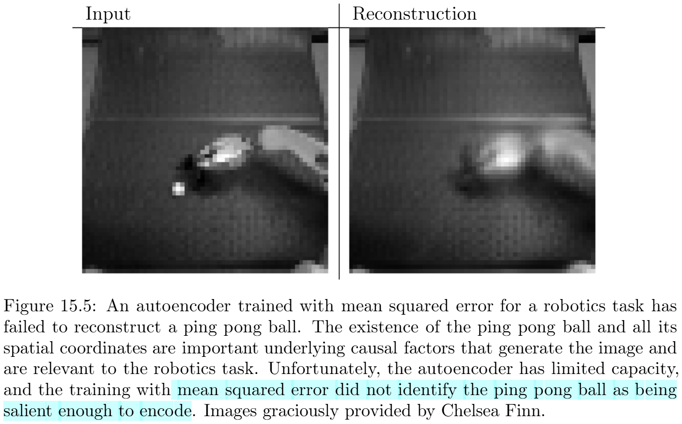
From the Deep Learning book (Goodfellow, Bengio, Courville)

Minimizing mean squared error in pixel space is similar to PCA, it mainly captures the directions of most variation (in pixel space). This does not necessarily mean it captures the semantically meaningful features. Is there some other way we can learn representations without manual labelling?

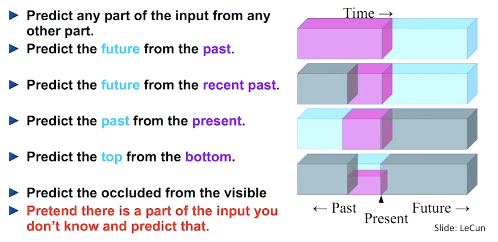
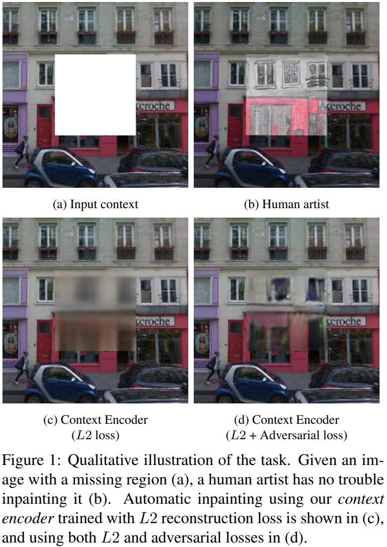
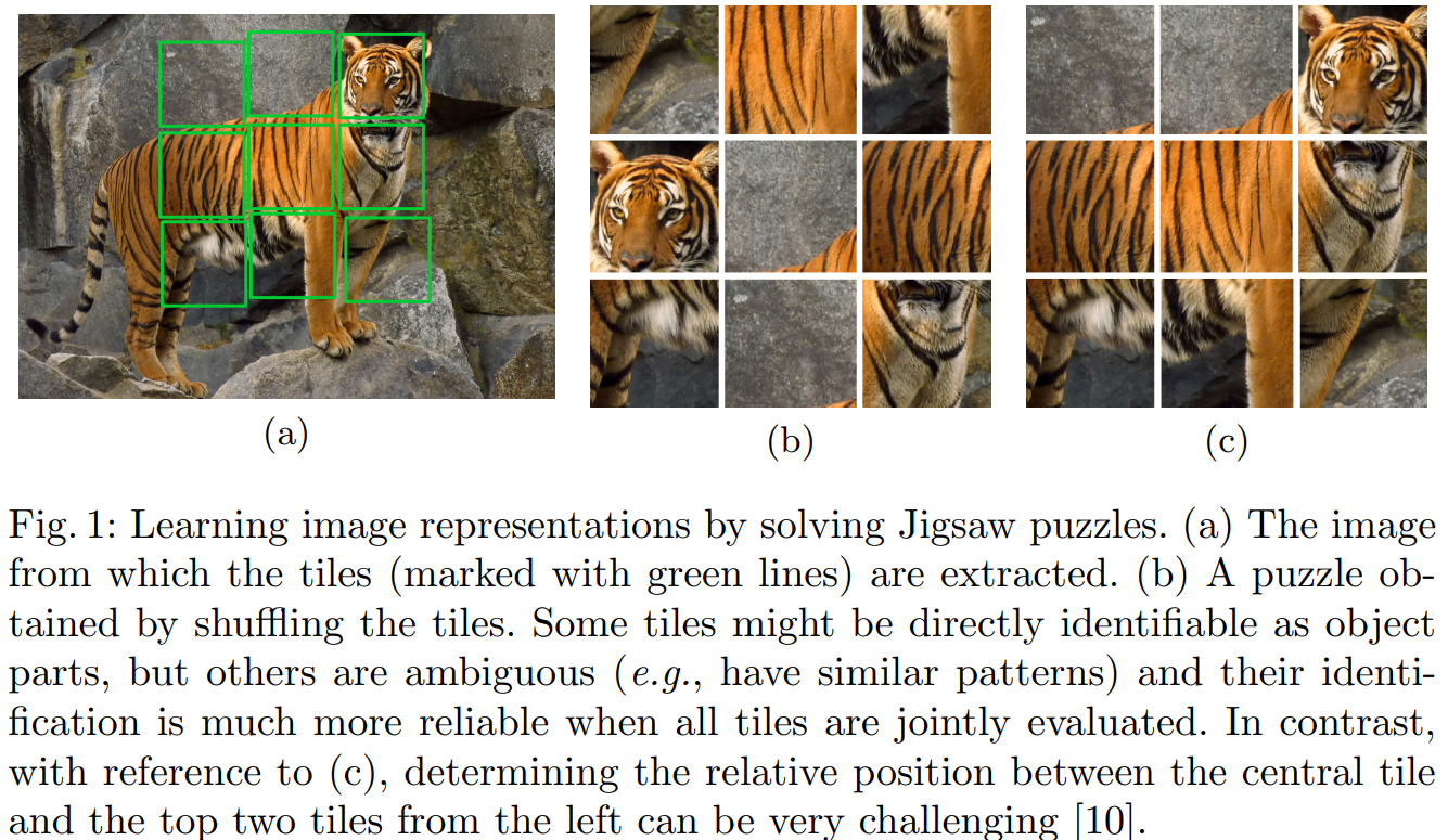
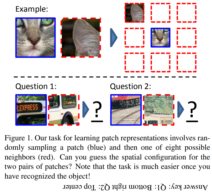
Self-supervised examples - predict in context

Pathak, Deepak, et al. “Context encoders: Feature learning by inpainting.” Proceedings of the IEEE conference on computer vision and pattern recognition. 2016.

Noroozi, Mehdi, and Paolo Favaro. “Unsupervised learning of visual representations by solving jigsaw puzzles.” European conference on computer vision. Cham: Springer International Publishing, 2016.

Doersch, Carl, Abhinav Gupta, and Alexei A. Efros. “Unsupervised visual representation learning by context prediction.” Proceedings of the IEEE international conference on computer vision. 2015.

Figure 1

Constrastive self-supervised learning

• Instead of relying on existing positive pairs, we can create them
• As long as the pairs we create have a semantic association, there is something to learn
• SimCLR is a very successful example of this

Chen, Ting, et al. “A simple framework for contrastive learning of visual representations.” International conference on machine learning. PmLR, 2020.

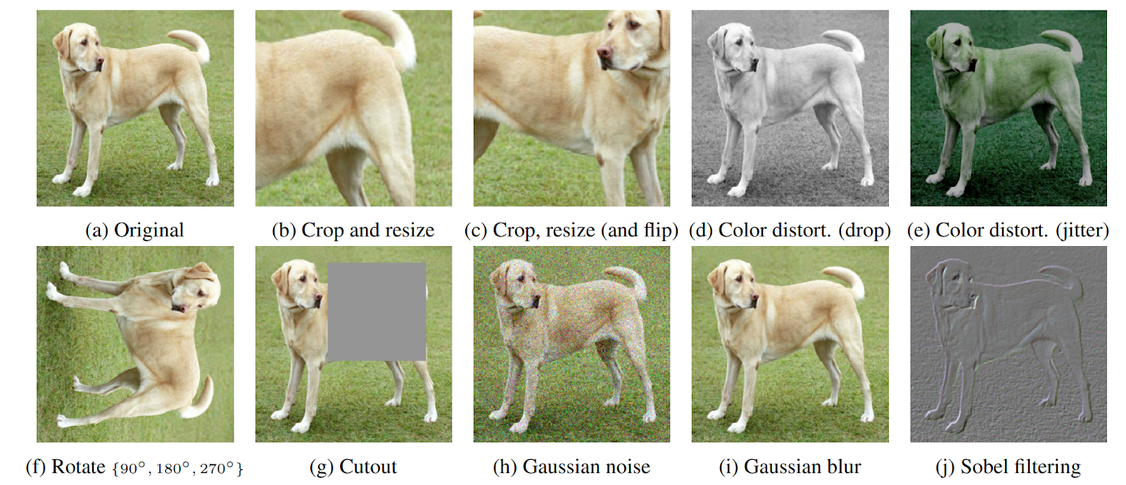
SimCLR - Findings

• Finding 1: The combinations of image transformations used to generate corresponding views are critical.

We found that while no single transformation (that we studied) suffices to define a prediction task that yields the best representations, two transformations stand out: random cropping and random color distortion. Although neither cropping nor color distortion leads to high performance on its own, composing these two transformations leads to state-of-the-art results.

• Finding 2: The nonlinear projection is important

In our experiments, we found that using such a nonlinear projection helps improve the representation quality, improving the performance of a linear classifier trained on the SimCLR-learned representation by more than 10%.

• Finding 3: Scaling up significantly improves performance.

we observe that the performance of a supervised ResNet peaked between 90 and 300 training epochs (on ImageNet), but SimCLR can continue its improvement even after 800 epochs of training

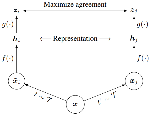
SimCLR — NT-Xent loss

For each image, SimCLR creates two augmented views (x_i, x_j), encodes and projects both to get normalised embeddings z_i, z_j. The NT-Xent (Normalised Temperature-scaled Cross-Entropy) loss asks the model to identify the matching view among all 2(N-1) other views in the batch:

\mathcal{L}^{\text{NT-Xent}}_{i,j} = -\log \frac{\exp\!\bigl(\operatorname{sim}(z_i, z_j)/\tau\bigr)}{\displaystyle\sum_{k=1}^{2N} \mathbf{1}_{[k \neq i]}\, \exp\!\bigl(\operatorname{sim}(z_i, z_k)/\tau\bigr)}

Symbol	Meaning
z_i = g(f(x_i))	Projected embedding: encoder f followed by projection head g
\operatorname{sim}(u,v) = u^\top v / (\|u\|\|v\|)	Cosine similarity
N	Batch size; 2N total views per batch
\tau	Temperature: lower \tau sharpens the distribution
\mathbf{1}_{[k \neq i]}	Excludes the anchor itself from the denominator

• The numerator rewards high similarity to the positive view.
• The denominator treats all 2N-2 other views as implicit negatives — no explicit pair selection needed.
• A large batch size is critical: more negatives in the denominator means a harder, more informative task.

Chen, Ting, et al. “A simple framework for contrastive learning of visual representations.” ICML, 2020.

Beyond contrastive learning

• The central part of contrastive learning is to bring associated examples close together
• Why do we need negative examples?
  • To avoid representational collapse

Tangent - Knowledge distillation

Instead of training a neural network (student) on the “hard” labels of our dataset, add “soft” targets from a really good (teacher) model.

Prakhar Ganesh, “Knowledge Distillation : Simplified”, https://towardsdatascience.com/knowledge-distillation-simplified-dd4973dbc764/

BYOL - Bootstrap your own latents

• Instead of avoiding representation collapse by using negative contrastive examples, what if we have two different models?
  • The main network we try to train – the online network
  • Another network we use to create the representations – the target network

Grill, Jean-Bastien, et al. “Bootstrap your own latent - a new approach to self-supervised learning.” Advances in neural information processing systems 33 (2020): 21271-21284.

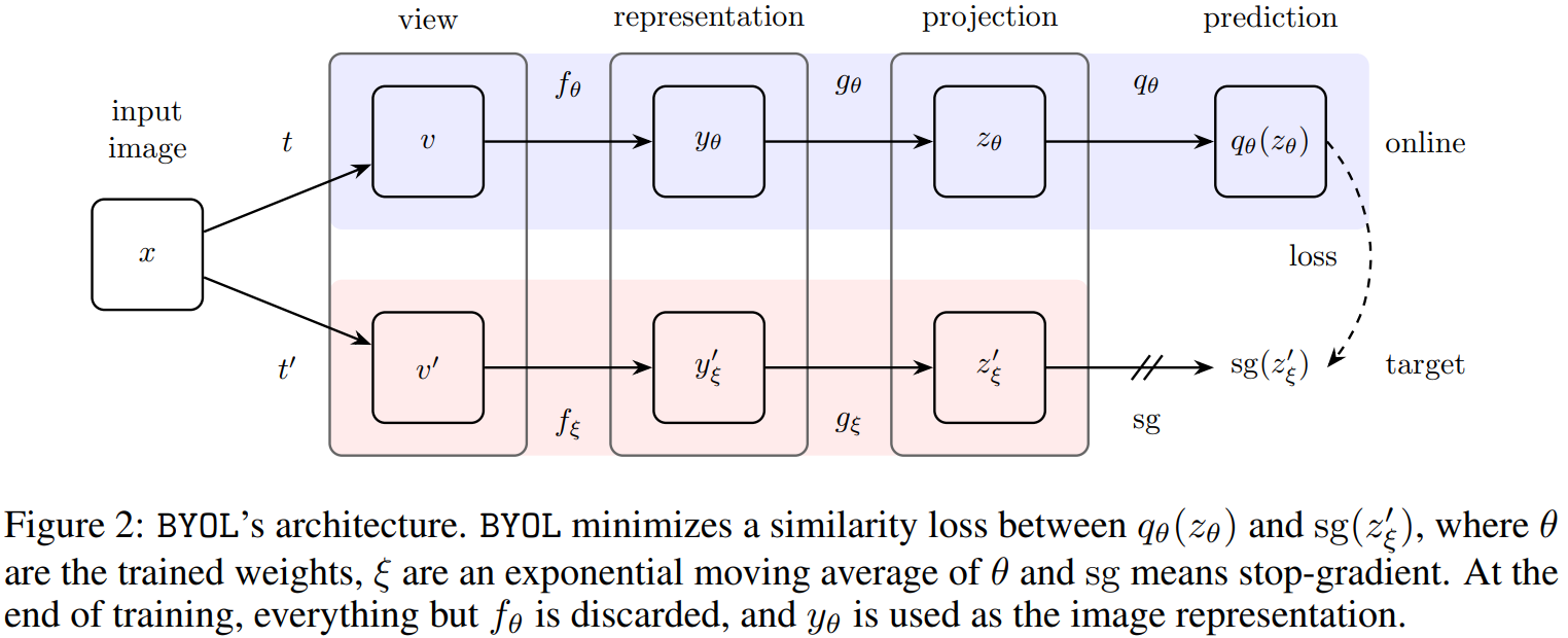
BYOL — loss and update rule

BYOL trains an online network (parameters \theta) to predict the representations of a target network (parameters \xi). There are no negative pairs; collapse is prevented by the asymmetry between the two networks.

\mathcal{L}_\text{BYOL} = \bigl\|\bar{q}_\theta(z^\text{online}) - \bar{z}^\text{target}\bigr\|_2^2 = 2 - 2\,\frac{\langle q_\theta(z^\text{online}),\, z^\text{target}\rangle}{\|q_\theta(z^\text{online})\|_2\;\|z^\text{target}\|_2}

Symbol	Meaning
z^\text{online} = g_\theta(f_\theta(x))	Online projection: encoder + projection head
z^\text{target} = g_\xi(f_\xi(x'))	Target projection for a different augmented view x'
q_\theta(\cdot)	Online predictor head (extra MLP absent from target network)
\bar{v} = v / \|v\|_2	L2-normalised vector
\xi \leftarrow \lambda\,\xi + (1-\lambda)\,\theta	Target updated via EMA — no gradient flows through it

• The predictor q_\theta creates the key asymmetry: the target has no predictor, so the online network must actively predict rather than just copy, preventing trivial collapse.
• The EMA target acts as a slowly evolving, consistent supervision signal — a “momentum encoder”.

Grill, Jean-Bastien, et al. “Bootstrap your own latent.” NeurIPS, 2020.

DINO = BYOL + Vision Transformers

Caron, Mathilde, et al. “Emerging properties in self-supervised vision transformers.” Proceedings of the IEEE/CVF international conference on computer vision. 2021.

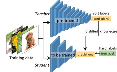
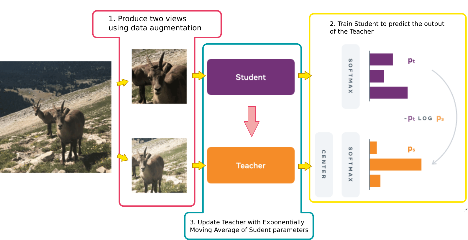
DINO — self-distillation loss

DINO uses a self-distillation objective: the student learns to match the (sharper) teacher’s output distribution over a set of learned prototype dimensions.

P_s(x) = \operatorname{softmax}\!\!\left(\frac{f_s(x)}{\tau_s}\right),\qquad P_t(x) = \operatorname{softmax}\!\!\left(\frac{f_t(x) - c}{\tau_t}\right)

\mathcal{L}_\text{DINO} = \sum_{\substack{v_1,\, v_2 \,\in\, \mathcal{V} \\ v_1 \neq v_2}} H\!\bigl(P_t(v_1),\, P_s(v_2)\bigr), \qquad H(p,q) = -\sum_i p_i \log q_i

Symbol	Meaning
\tau_s > \tau_t	Student temperature higher — teacher output is sharper (more confident)
c	Centering vector: EMA of teacher outputs, subtracted to prevent one-prototype collapse
\mathcal{V}	Multi-crop views: 2 global + several local crops
\theta_t \leftarrow m\,\theta_t + (1-m)\,\theta_s	Teacher updated by EMA only — no backprop through teacher

• Global-to-local consistency: teacher sees only global crops; student sees local crops too — forcing the student to infer global structure from a small patch.
• Collapse is prevented by two complementary mechanisms: centering (shifts teacher logits) and sharpening (low \tau_t makes teacher peaked).

Caron, Mathilde, et al. “Emerging properties in self-supervised vision transformers.” ICCV, 2021.

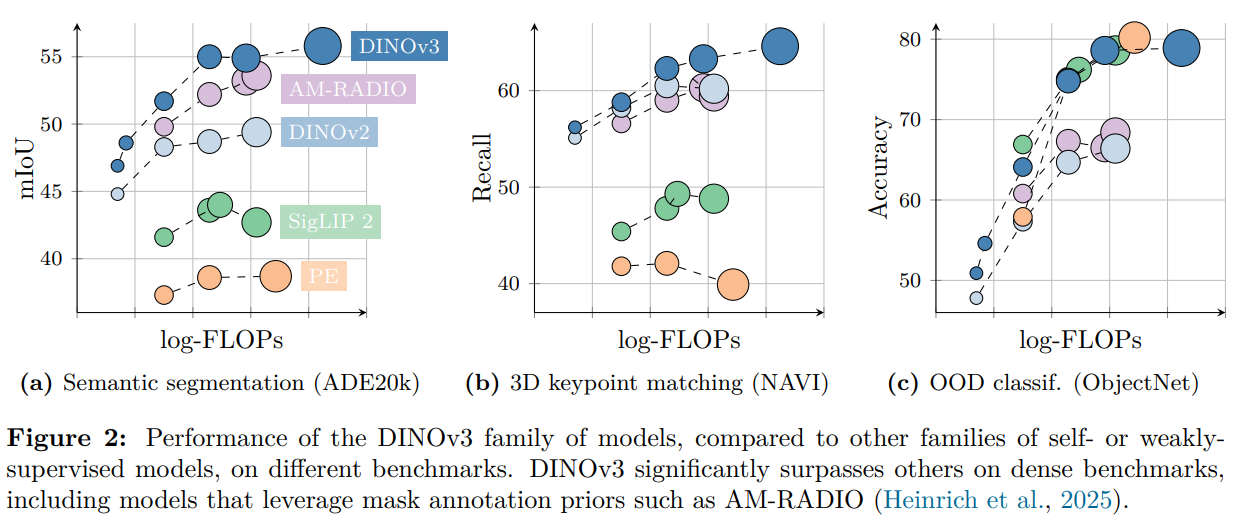
DINO v3

• Development of DINO v2 to increase model scale
  • Large data with auto curation
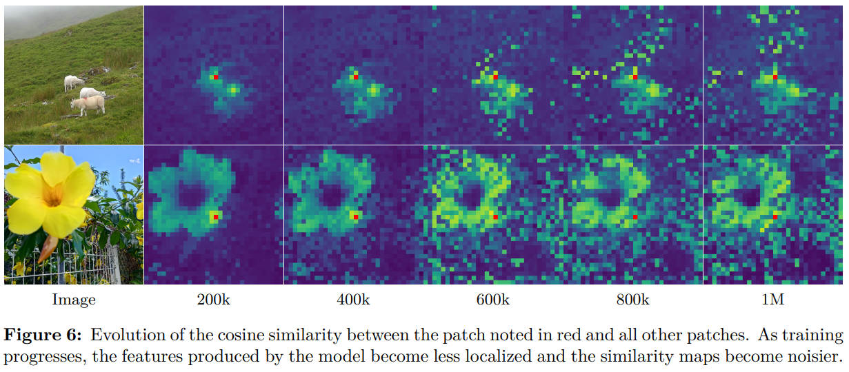
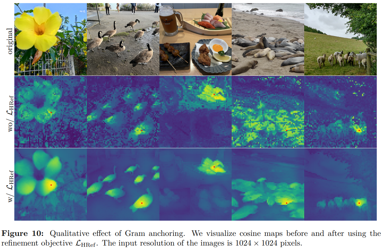
  • Regularized patch representations with Gram matching

Siméoni, Oriane, et al. “Dinov3.” arXiv preprint arXiv:2508.10104 (2025).

for images have been hard - Models are unstable in terms of performance - Coherence of attention maps degrade over training time - DINO v3 introduces a series of tricks to improve this - Automated data curation - train on larger sets of data with higher average quality - Starts from a pool of 17B images from Instagram, clusters and chooses balanced coverage to 1689 million images - Tweaks to architecture (positional embeddings) - Regularizing the attention maps (Gram matching) - Match matrix of pairwise dot products of all patches to a example from early on in training (regularizing the feature structure, keeping it spread oout) - Scaling up SSL methods like DINO (in terms of model size) for images have been hard - Models are unstable in terms of performance - Coherence of attention maps degrade over training time - DINO v3 introduces a series of tricks to improve this

DINO v3 - Gram matching

Figure 2: Siméoni, Oriane, et al. “Dinov3.” arXiv preprint arXiv:2508.10104 (2025).

\mathcal{L}_\text{Gram} = \lVert \mathbf{X}_S \cdot \mathbf{X}_S^\top - \mathbf{X}_G \cdot \mathbf{X}_G^\top \rVert_\text{F}^2

Constrain all the pairs of inner products to be similar to an earlier version of the model

for images have been hard - Models are unstable in terms of performance - Coherence of attention maps degrade over training time - DINO v3 introduces a series of tricks to improve this - Automated data curation - train on larger sets of data with higher average quality - Starts from a pool of 17B images from Instagram, clusters and chooses balanced coverage to 1689 million images - Tweaks to architecture (positional embeddings) - Regularizing the attention maps (Gram matching) - Match matrix of pairwise dot products of all patches to a example from early on in training (regularizing the feature structure, keeping it spread oout) - Scaling up SSL methods like DINO (in terms of model size) for images have been hard - Models are unstable in terms of performance - Coherence of attention maps degrade over training time - DINO v3 introduces a series of tricks to improve this

Multimodal Learning

Multimodal Machine Learning tutorial - ACL2017 – https://www.cs.cmu.edu/~morency/MMML-Tutorial-ACL2017.pdf

Use modalities to label each other

With supervised contrastive learning we need to label the data

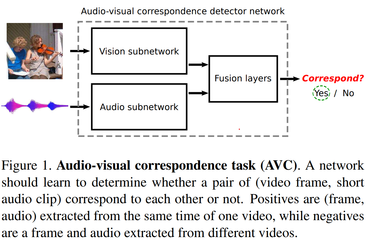
Arandjelovic, Relja, and Andrew Zisserman. “Look, listen and learn.” Proceedings of the IEEE International Conference on Computer Vision. 2017.

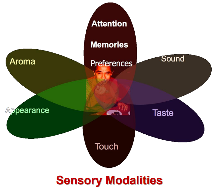
With multimodal data we have “natural” associations in the separate modalities.

Use modalities to label each other

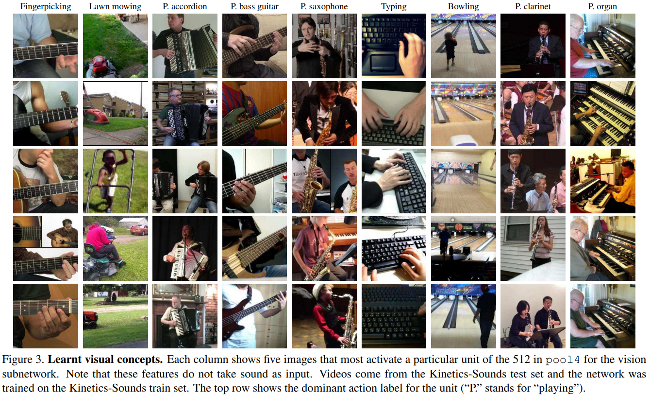
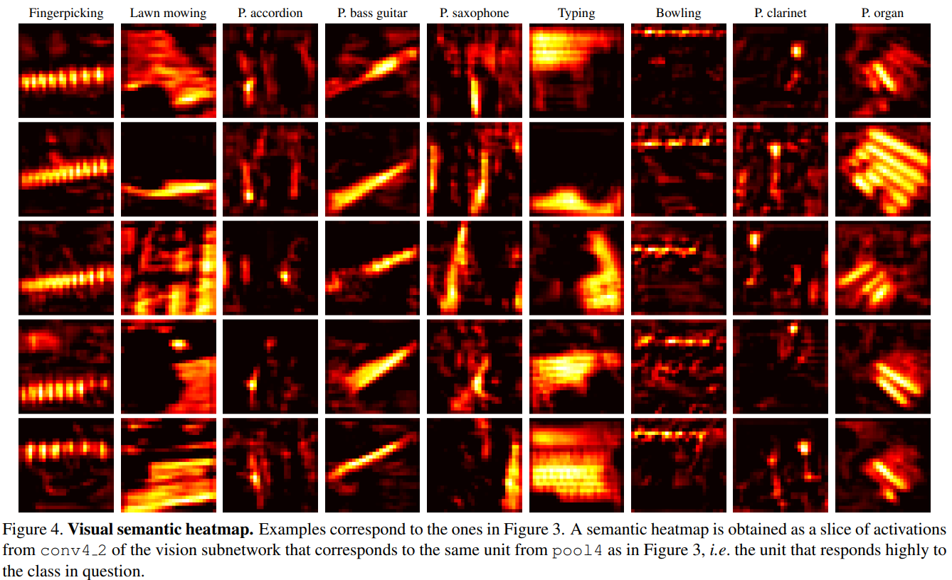
Figure 3: Arandjelovic, Relja, and Andrew Zisserman. “Look, listen and learn.” Proceedings of the IEEE International Conference on Computer Vision. 2017. za

Use modalities to label each other

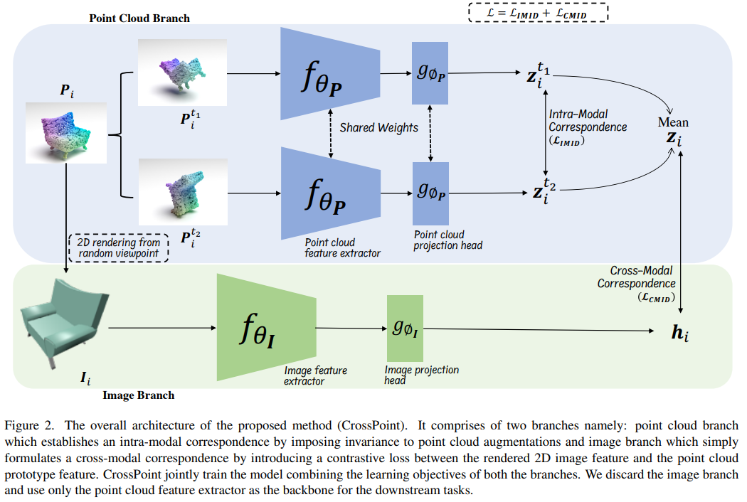
Afham, Mohamed, et al. “Crosspoint: Self-supervised cross-modal contrastive learning for 3d point cloud understanding.” Proceedings of the IEEE/CVF conference on computer vision and pattern recognition. 2022.

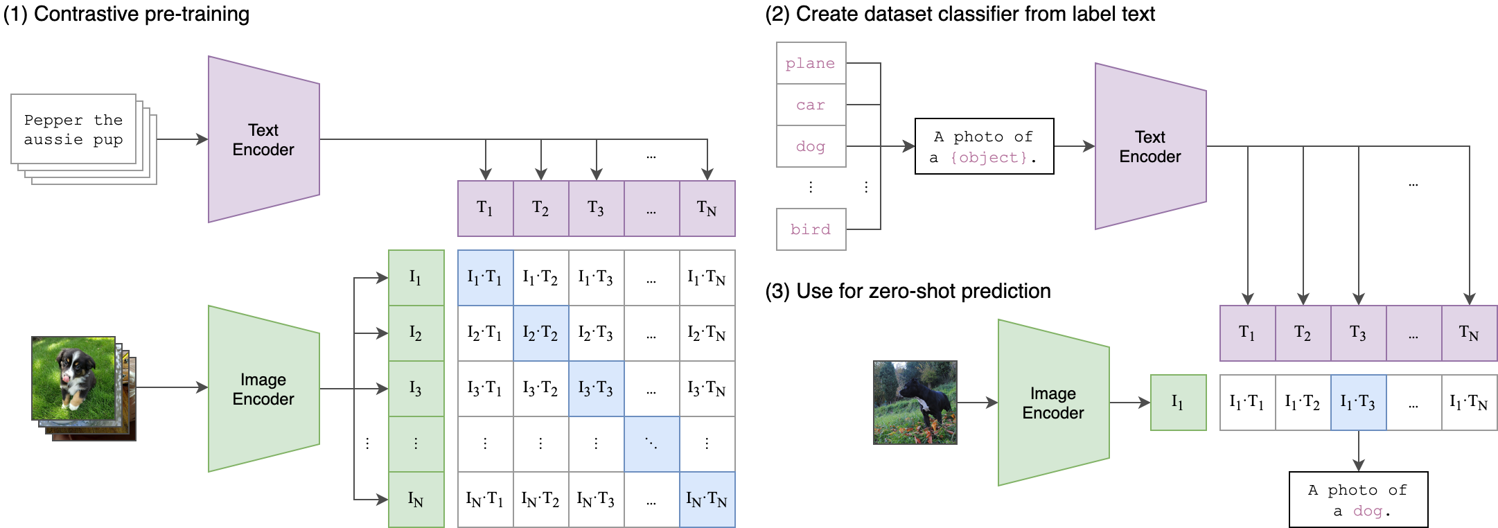
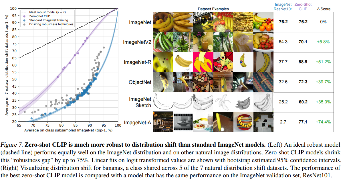
CLIP

https://github.com/openai/CLIP

CLIP

Radford, Alec, et al. “Learning transferable visual models from natural language supervision.” International Conference on Machine Learning. PMLR, 2021.

CLIP — symmetric contrastive loss

For a batch of N image–text pairs, CLIP computes L2-normalised embeddings from two separate encoders and applies a symmetric NT-Xent loss across modalities:

\mathcal{L}_\text{CLIP} = \frac{1}{2}\Bigl(\mathcal{L}_{I \to T} + \mathcal{L}_{T \to I}\Bigr)

\mathcal{L}_{I \to T} = -\frac{1}{N}\sum_{i=1}^N \log \frac{\exp(I_i \cdot T_i\,/\,\tau)}{\displaystyle\sum_{j=1}^N \exp(I_i \cdot T_j\,/\,\tau)}, \qquad \mathcal{L}_{T \to I} = -\frac{1}{N}\sum_{i=1}^N \log \frac{\exp(T_i \cdot I_i\,/\,\tau)}{\displaystyle\sum_{j=1}^N \exp(T_j \cdot I_i\,/\,\tau)}

CLIP symbol description

Symbol	Meaning
I_i = f_I(x_i) / \|f_I(x_i)\|	L2-normalised image embedding
T_i = f_T(c_i) / \|f_T(c_i)\|	L2-normalised text embedding for paired caption c_i
\tau	Learned temperature (not a fixed hyperparameter as in SimCLR)

Radford, Alec, et al. “Learning transferable visual models from natural language supervision.” ICML, 2021.

CLIP — symmetric contrastive loss

For a batch of N image–text pairs, CLIP computes L2-normalised embeddings from two separate encoders and applies a symmetric NT-Xent loss across modalities:

\mathcal{L}_\text{CLIP} = \frac{1}{2}\Bigl(\mathcal{L}_{I \to T} + \mathcal{L}_{T \to I}\Bigr)

\mathcal{L}_{I \to T} = -\frac{1}{N}\sum_{i=1}^N \log \frac{\exp(I_i \cdot T_i\,/\,\tau)}{\displaystyle\sum_{j=1}^N \exp(I_i \cdot T_j\,/\,\tau)}, \qquad \mathcal{L}_{T \to I} = -\frac{1}{N}\sum_{i=1}^N \log \frac{\exp(T_i \cdot I_i\,/\,\tau)}{\displaystyle\sum_{j=1}^N \exp(T_j \cdot I_i\,/\,\tau)}

Relation to SimCLR and SupCon:

• vs SimCLR: identical NT-Xent structure — one positive per anchor, all others are implicit negatives — but the “two views” come from different modalities rather than image augmentations. The loss is also symmetrised (both I \to T and T \to I).
• vs SupCon: each anchor has exactly |P(i)| = 1 positive (its paired caption), making it the single-positive special case of SupCon. Scaling to very large batches gives the same benefit SupCon gets from many in-batch positives: a rich, continuous repulsion against all other examples.
• The key novelty is using natural image–language pairing as supervision — no augmentation strategy needed, just internet-scale (image, caption) pairs.

Radford, Alec, et al. “Learning transferable visual models from natural language supervision.” ICML, 2021.

Summary

• Contrastive learning is a general technique for learning representations
• Self-supervised learning is about crafting ways of learning from unlabeled data
• Clever augmentations technique can use contrastive learning without labled data
• Multimodal data is perfect for contrastive learning, the modalities “label each other”