Convolutional Neural Networks for Image Segmentation

Localisation, detection, and segmentation

Christophe Avenel

NBIS

08-May-2026

CNNs for computer vision

Some of the material from this lecture comes from online courses of Charles Ollion and Olivier Grisel - Master Datascience Paris Saclay. CC-By 4.0 license.

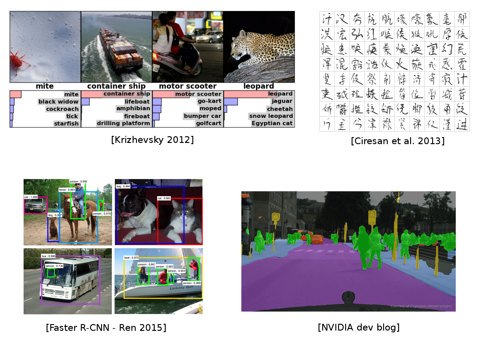
Beyond image classification

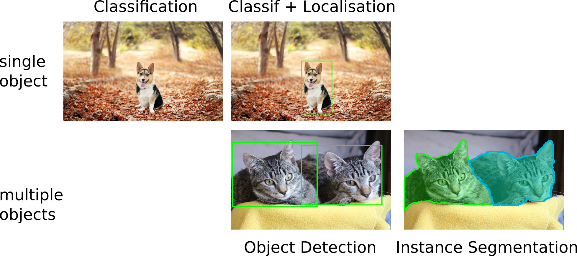
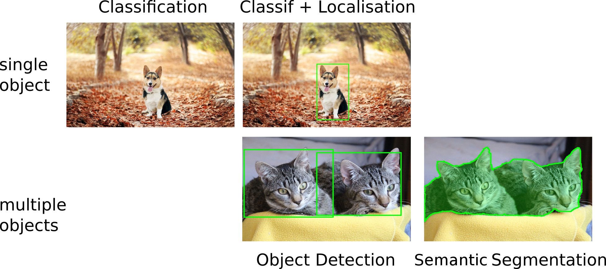
Classification answers “what is in this image?” — but real-world vision asks more:

• Where is the object? (localisation)
• How many objects, and which class is each one? (detection)
• Which pixels belong to which object? (segmentation)

From classification to dense prediction

• Same backbone (CNN/ViT) — but with task-specific heads
• The pretrained classifier is the starting point in (almost) every modern approach

Outline

• Localisation as regression
• Detection algorithms (YOLO, RetinaNet, Faster R-CNN)
• Fully convolutional networks → U-Net
• Losses and transfer learning for segmentation
• Instance segmentation (Mask R-CNN) and what came after

Localisation

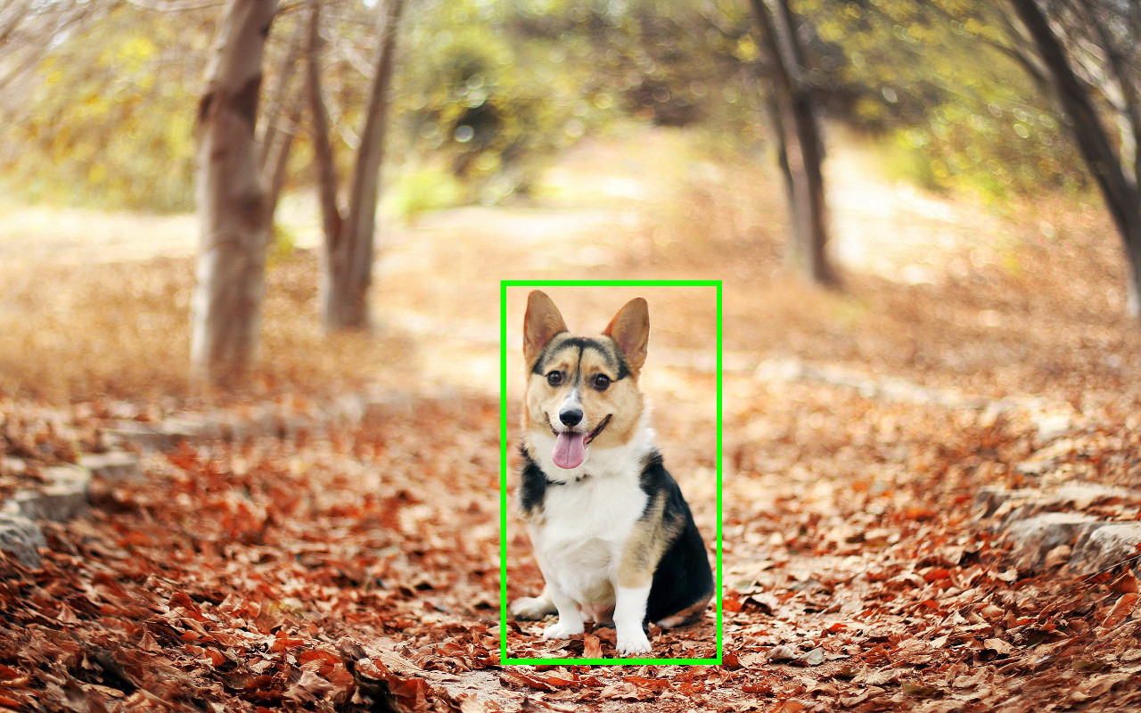
• Single object per image
• Predict coordinates of a bounding box (x, y, w, h)
• Evaluate via Intersection over Union (IoU)

Localisation as regression

Classification + Localisation

• Use a pre-trained CNN on ImageNet (e.g. ResNet)
• The “localisation head” is trained separately with regression
• At test time, use both heads

C classes, 4 output dimensions (1 box)

Predict exactly N objects: predict (N \times 4) coordinates and (N \times K) class scores

Object detection

We don’t know in advance the number of objects in the image. Object detection relies on object proposal and object classification:

• Object proposal: find regions of interest (RoIs) in the image
• Object classification: classify the object in these regions

Two main families

• Single-Stage: a grid in the image where each cell is a proposal (SSD, YOLO, RetinaNet)
• Two-Stage: region proposal then classification (Faster-RCNN)

YOLO (You Only Look Once)

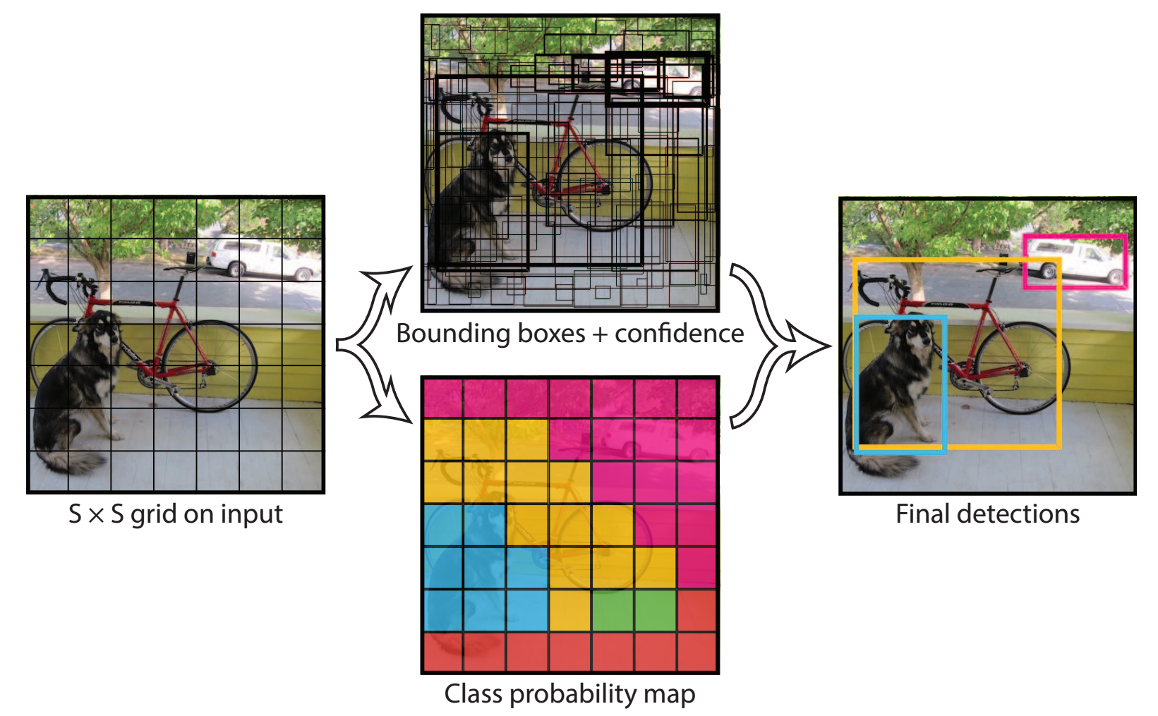
For each cell of the S \times S grid predict:

• B boxes and confidence scores C (5 \times B values) + classes c
• Final detections: C_j \cdot \mathrm{prob}(c) > \text{threshold}

• One CNN, one forward pass — real-time detection
• Globally processes the entire image at once

Redmon et al. “You only look once: Unified, real-time object detection.” CVPR 2016. The single-shot grid is still the conceptual core, even if modern YOLO versions add anchor-free heads, FPN, decoupled heads, etc.

YOLO today

The original YOLO concept is now a mature production library maintained by Ultralytics.

from ultralytics import YOLO

model = YOLO("yolo11n.pt")          # COCO-pretrained, ~3 MB
results = model.predict("img.jpg")   # detection
results = model.predict("img.jpg", task="segment")  # instance segmentation

• Current generation: YOLOv11 (2024) — anchor-free, decoupled heads, FPN
• One package covers detection, instance segmentation, pose estimation, OBB, tracking
• Real-time on CPU for the small variants; GPU for bigger ones

RetinaNet

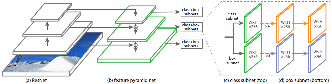
Single stage detector with:

• Multiple scales through a Feature Pyramid Network
• More than 100K boxes proposed
• Focal loss to manage imbalance between background and real objects

See this post for more information.

Lin, Tsung-Yi, et al. “Focal loss for dense object detection.” ICCV 2017.

Box Proposals

Instead of using a predefined set of box proposals, find them on the image:

• Selective Search — from pixels (not learnt)
• Faster R-CNN — Region Proposal Network (RPN)

Crop-and-resize operator (RoI-Pooling):

• Input: convolutional map + N regions of interest
• Output: tensor of N \times 7 \times 7 \times \text{depth} boxes
• Allows the gradient to propagate only on interesting regions, and efficient computation

Faster R-CNN

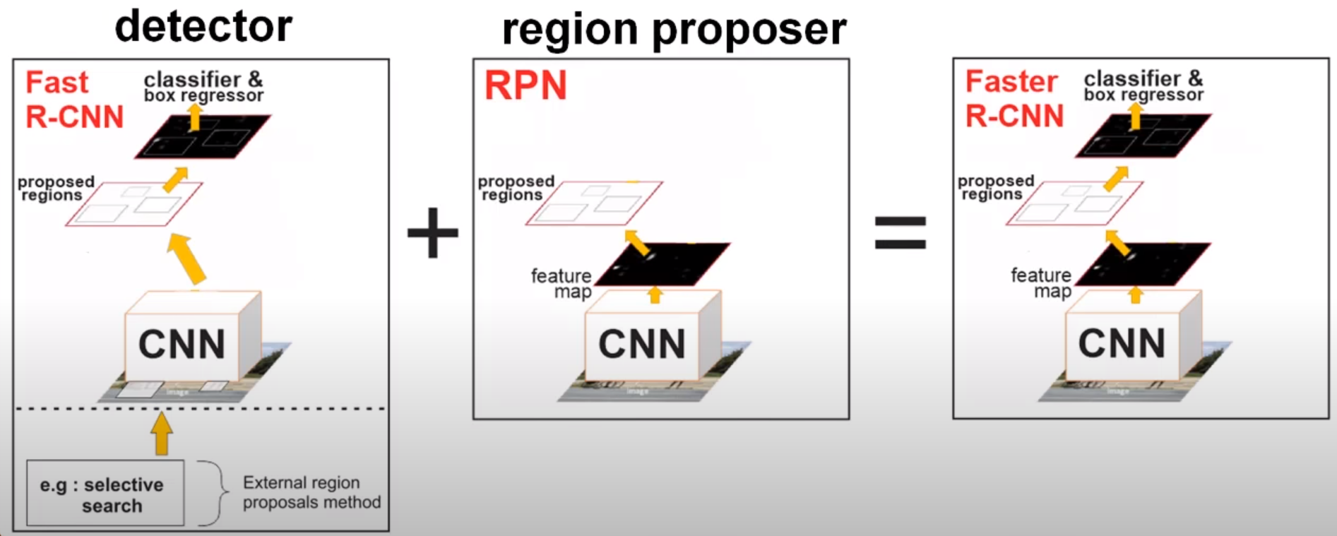
• Replace Selective Search with RPN, train jointly
• Region proposal is translation invariant, compared to YOLO

Ren, Shaoqing, et al. “Faster r-cnn: Towards real-time object detection with region proposal networks.” NIPS 2015

Segmentation

Output a class map for each pixel (here: dog vs background).

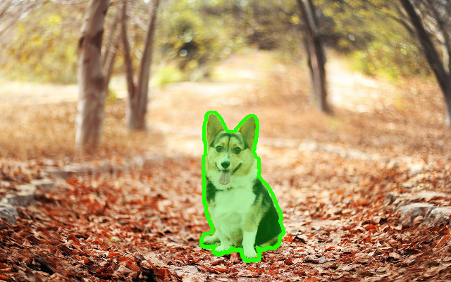
• Instance segmentation: specify each object instance as well (two dogs have different instances)
• This can be done through object detection + segmentation

Convolutionize

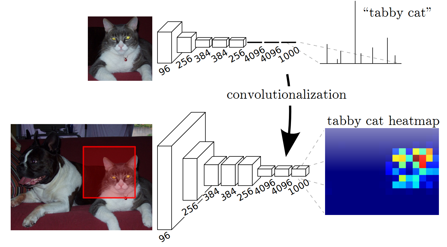
• Slide the network with an input of (224, 224) over a larger image. Output of varying spatial size
• Convolutionize: change Dense (4096, 1000) to 1 \times 1 Convolution, with 4096, 1000 input and output channels
• Gives a coarse segmentation (no extra supervision)

Long, Jonathan, et al. “Fully convolutional networks for semantic segmentation.” CVPR 2015

Fully Convolutional Network

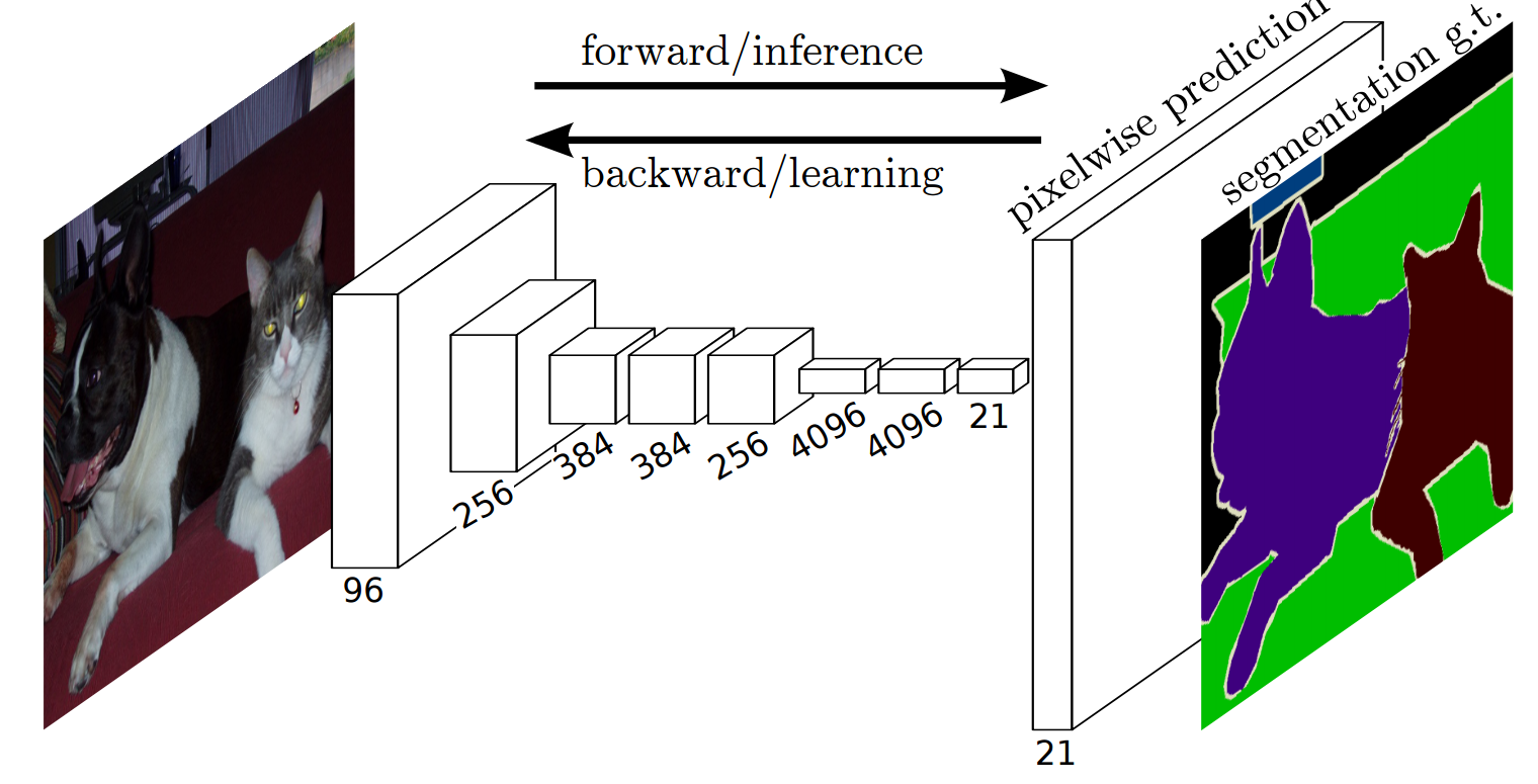
• Predict / backpropagate for every output pixel
• Aggregate maps from several convolutions at different scales for more robust results

Long, Jonathan, et al. “Fully convolutional networks for semantic segmentation.” CVPR 2015

Deconvolution

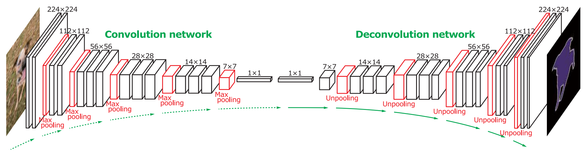
“Deconvolution”: transposed convolutions

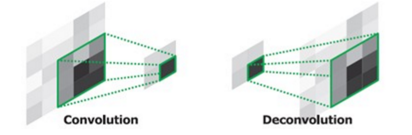
Noh, Hyeonwoo, et al. “Learning deconvolution network for semantic segmentation.” ICCV 2015

U-Net

• Symmetric encoder–decoder with skip connections that concatenate features from the contracting path to the expanding path
• Trains well on small datasets with heavy augmentation
• Fully convolutional → arbitrary input sizes at inference
• The default architecture for biomedical and microscopy segmentation — directly relevant to the lab

Ronneberger, Fischer, Brox. “U-Net: Convolutional Networks for Biomedical Image Segmentation.” MICCAI 2015. Skip connections concatenate (not add, as in ResNet) to preserve spatial detail through the bottleneck.

Segmentation losses

Segmentation = per-pixel classification, but with a strong class-imbalance problem (background dominates).

• Cross-entropy (per pixel) — the default, but biased toward the majority class
• Dice loss — directly optimizes overlap with the ground-truth mask:

\mathcal{L}_{\text{Dice}} = 1 - \frac{2 \, |P \cap G|}{|P| + |G|}

• Focal loss — down-weights easy pixels, focuses on hard ones (same idea as RetinaNet, applied per-pixel)

In practice for biomedical/microscopy: train with BCE + Dice (sum of the two) for stable convergence on imbalanced masks.

Transfer learning for segmentation

Same recipe as classification: pretrained encoder + task-specific decoder.

import segmentation_models_pytorch as smp

model = smp.Unet(
    encoder_name="resnet34",       # any timm/torchvision backbone
    encoder_weights="imagenet",    # ImageNet-pretrained
    in_channels=1,                  # grayscale microscopy
    classes=5,                      # number of mask channels
)

• Decoder is randomly initialized; encoder starts from ImageNet weights
• Works even when the input domain (microscopy, satellite, MRI) differs from ImageNet
• Same library exposes U-Net, FPN, DeepLabV3+, MA-Net, etc. Swap one string

Mask R-CNN

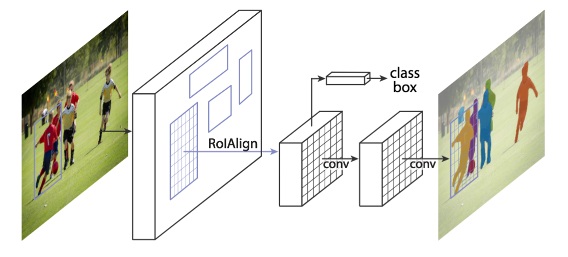
Faster R-CNN architecture with a third, binary mask head.

K. He et al. Mask Region-based Convolutional Network (Mask R-CNN) NIPS 2017

Mask R-CNN: Results

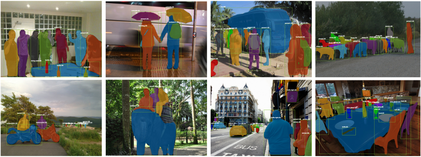
• Mask results are still coarse (low mask resolution)
• Excellent instance generalization

K. He et al. Mask R-CNN. NIPS 2017

What came after Mask R-CNN

Year	Model	Key idea
2020	DETR	Transformer detection, end-to-end, no anchors / no NMS
2022	Mask2Former	Unified semantic / instance / panoptic segmentation
2023	SAM	Promptable segmentation: “click and get a mask”
2024	SAM 2	SAM extended to video with temporal consistency

Foundation models for segmentation (SAM 2, Grounding DINO, …): pretrained on billions of masks, often zero-shot for new domains.

Summary

• Localisation: regression heads on a CNN backbone for (x, y, w, h)
• Detection: single-stage (YOLO, RetinaNet) vs. two-stage (Faster R-CNN); modern YOLO is a one-line pip install
• Segmentation: encoder–decoder with skip connections, U-Net is the workhorse for biomedical imaging
• Train it right: pretrained encoder + BCE + Dice loss + augmentation
• Instance segmentation: Mask R-CNN, then DETR / Mask2Former
• Today: foundation models (SAM 2, Grounding DINO) often give zero-shot masks.

Next: hands-on segmentation lab on biological images, where U-Net + Dice loss is the natural baseline.