Convolutional Neural Networks for Image Classification
From convolutions to modern architectures
Christophe Avenel
NBIS
08-May-2026
CNNs for computer vision
Some of the material from this lecture comes from online courses of Charles Ollion and Olivier Grisel — Master Datascience Paris Saclay. CC-By 4.0 license.
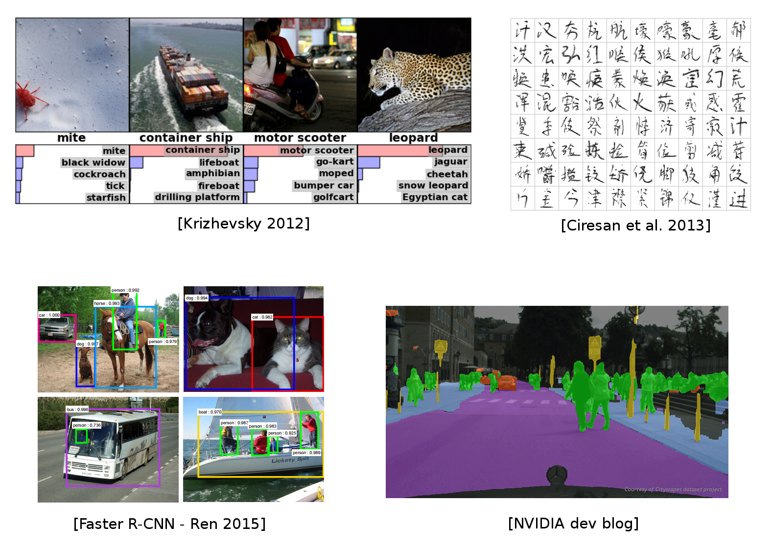
CNN for image classification
CNN = Convolutional Neural Networks (or ConvNets)
LeCun, Y., Bottou, L., Bengio, Y., and Haffner, P. (1998). LeNet: gradient-based learning applied to document recognition.
Outline
Convolutions
Convolutions in Neural Networks
Motivations
Layers
Architectures
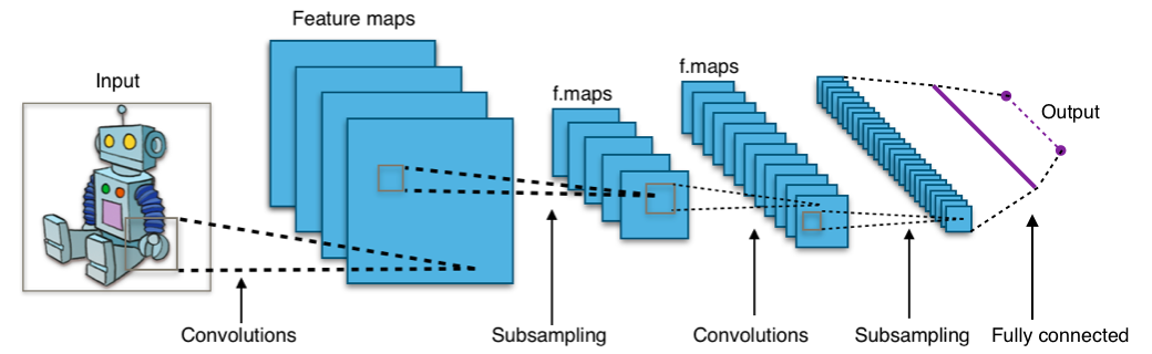
Classic CNN Architecture
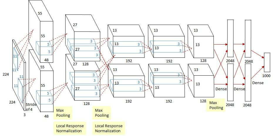
AlexNet
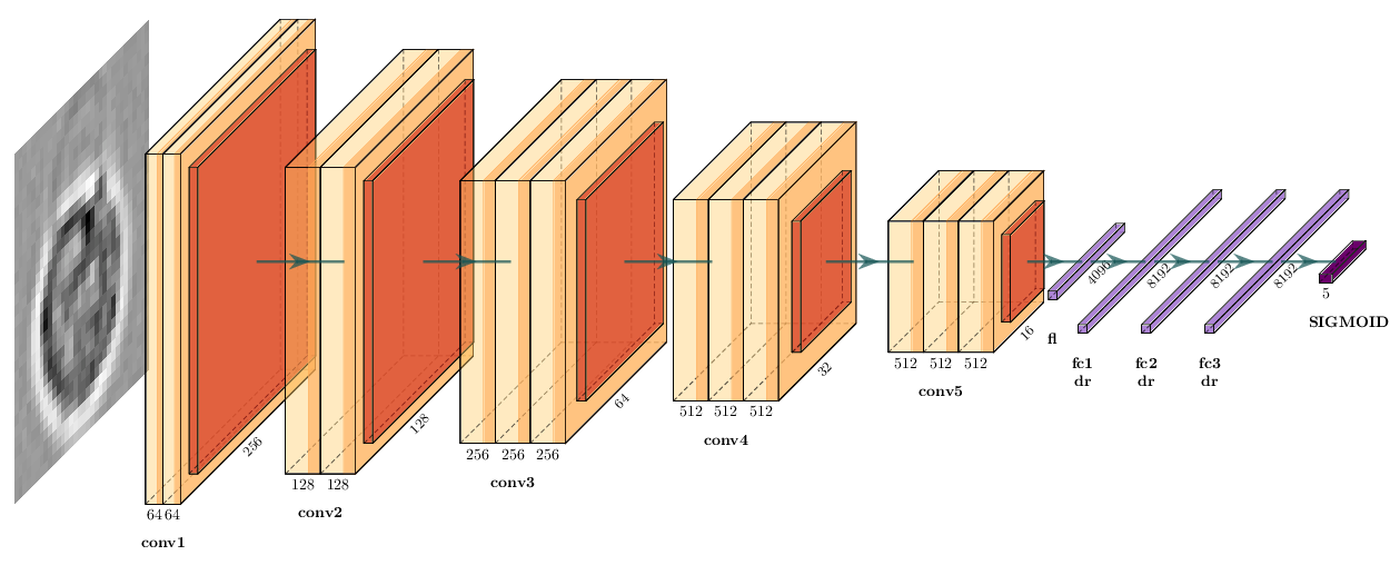
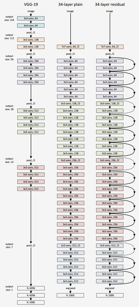
VGG16
ResNet
Convolution
A mathematical operation that combines two functions to form a third function.
The feature map (or input data) and the kernel are combined to form a transformed feature map.
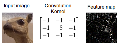
Often interpreted as a filter: the kernel filters the feature map for certain information (edges, etc.)
Convolving an image with an edge detector kernel.
The mathematical definition of the convolution of two functions f and x over a range t:
y(t) = f \otimes x = \int_{-\infty}^{\infty} f(k) \cdot x(t-k)\, \mathrm{d}k
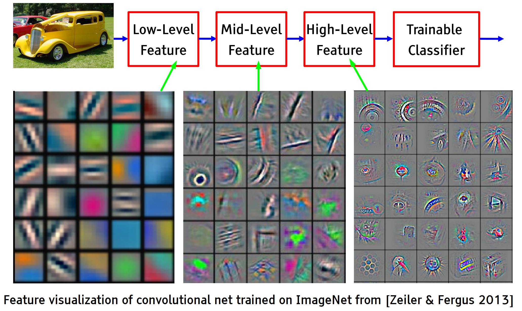
Convolutional filters can be interpreted as feature detectors:
The input (feature map) is filtered for a certain feature (the kernel).
The output is large if the feature is detected in the image.
The kernel can be interpreted as a feature detector where a detected feature results in large outputs (white) and small outputs if no feature is present (black).
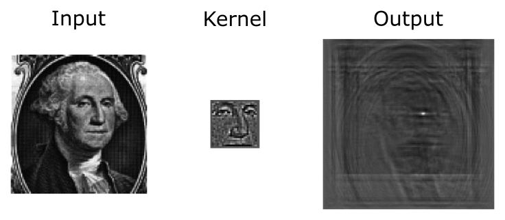
Image kernels demo
Interactive demo of image kernels from setosa.io.
Convolution in a neural network
x is a 3 \times 3 chunk (yellow area) of the image (green array)
Each output neuron is parametrized with the 3 \times 3 weight matrix \mathbf{w} (small numbers)
The activation is obtained by sliding the 3 \times 3 window and computing:
z(x) = \mathrm{relu}(\mathbf{w}^T x + b)
Motivations
Standard Dense Layer for an image input:
import torchimport torch.nn as nn# x: image batch of shape (N, 3, 480, 640)x = torch.randn(1, 3, 480, 640)y = nn.Flatten()(x)# shape of y is: (N, 3 * 480 * 640)z = nn.Linear(3*480*640, 1000)(y)
More advanced: MixUp / CutMix (mix images and labels)
Always validate/test on un-augmented images
Transfer learning
You almost never train a CNN from scratch. Start from ImageNet-pretrained weights:
from torchvision.models import resnet50, ResNet50_Weightsmodel = resnet50(weights=ResNet50_Weights.IMAGENET1K_V2)# Replace the classification head for your N classesmodel.fc = nn.Linear(model.fc.in_features, num_classes)# Optionally freeze the backbone (linear-probe) ...for p in model.parameters(): p.requires_grad =Falsefor p in model.fc.parameters(): p.requires_grad =True# ... or fine-tune the whole network with a small learning rate.
Linear probe: freeze backbone, train only the head (fast, small data)
Fine-tune: train everything with a small learning rate (best results, more data)
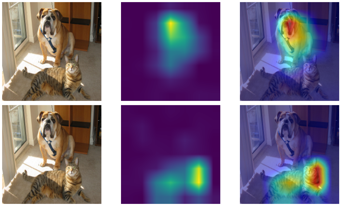
Class-specific saliency map, no architectural changes needed
Use it to spot shortcut learning (e.g. model attending to background, watermarks, scanner artefacts).
Selvaraju et al., “Grad-CAM: Visual Explanations from Deep Networks via Gradient-based Localization”, ICCV 2017. Available in PyTorch via the grad-cam package or as a ~30-line manual hook.
Most parameters live in the first FC layer — modern designs avoid this
Activations dominate memory at training time, parameters at inference time
Pattern: feature map size halves while channels double through pooling stages, until the dense head dominates parameter count. Modern nets replace those FC layers with global average pooling.
Counts include biases. Adam stores 2 extra moment buffers per parameter (≈ ×3 total memory); plain SGD with momentum stores 1 (≈ ×2).
ResNet
Even deeper models:
34, 50, 101, 152 layers
He, Kaiming, et al. “Deep residual learning for image recognition.” CVPR. 2016.
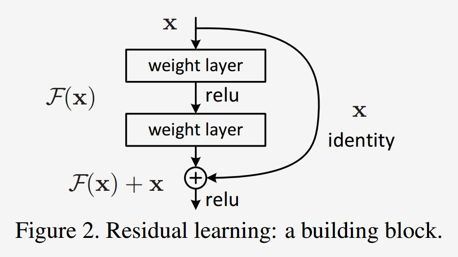
ResNet — residual blocks
A block learns the residual w.r.t. identity
Good optimization properties
ResNet vs. VGG
ResNet50 compared to VGG:
Superior accuracy in all vision tasks
5.25% top-5 error vs. 7.1%
Less parameters
25M vs. 138M
Computational complexity
3.8B Flops vs. 15.3B Flops
Fully Convolutional until the last layer
What came after ResNet (2017–today)
Year
Model
Key idea
2014
Inception
factorized convolutions (1×1 + 3×3 + 5×5)
2017
MobileNet
depthwise-separable convs for mobile / edge
2019
EfficientNet
compound scaling of width/depth/resolution
2020
ViT
image as a sequence of patches → Transformer
2022
ConvNeXt
“modernized” CNN, matches ViTs at same compute
Vision Transformers (ViT) and foundation models (CLIP, DINOv2, SAM 2) are now state-of-the-art for many tasks.
ImageNet-1k benchmarks
Model
Year
Params
Top-1
Notes
ResNet-50
2015
25 M
76.1%
the workhorse baseline
EfficientNet-B0
2019
5.3 M
77.7%
great accuracy/parameter
ConvNeXt-T
2022
29 M
82.1%
pure CNN, ViT-competitive
ViT-B/16
2020
86 M
81.1%
needs large-scale pretrain
ViT-L/16 + DINOv2
2023
300 M
86.7%
self-supervised pretraining
Architectures are converging at the top — CNN vs. Transformer matters less than data, scale, and pretraining
For most lab/research settings, a pretrained ResNet-50 or ConvNeXt-T is a strong default
Numbers are approximate, sourced from the torchvision / timm model zoos. Throughput depends heavily on hardware — exact figures less important than the trend.
Summary
Convolutions exploit local connectivity and parameter sharing to scale to images
Stacking conv + pooling layers builds a hierarchy of features
BatchNorm + residual connections were the key unlocks for very deep networks
Data augmentation is the cheapest regularizer; always use it
Today, start from pretrained weights — fine-tune or linear-probe rather than train from scratch
Use Grad-CAM to inspect what your model actually attends to
Coming up:
Next lecture — beyond classification: localisation, detection, segmentation