CNN Lab 2: Segmentation of Human Blood Cells using PyTorch

Pixel-wise classification of blood cell images with a U-Net in PyTorch, then the same task with a VGG16-backboned U-Net from segmentation_models_pytorch.

Author

Affiliation

Christophe Avenel

NBIS

Running on colab

To run this notebook on Google Colab:

Download the notebook from this link.
Go to colab.research.google.com, then File → Open notebook → Upload and select the downloaded file.
Make a copy to your own Google Drive before starting your work, so that your changes are saved.
Download and unzip the data by running the following in a new cell:

Code

!wget https://user.it.uu.se/~chrav452/workshop_NN_DL_cnn_data.zip
!unzip workshop_NN_DL_cnn_data.zip

Segmentation of Human Blood Cells using Convolutional Neural Networks

For this lab, we use the Human White Blood Cell images from Jiangxi Tecom Science Corporation, China.

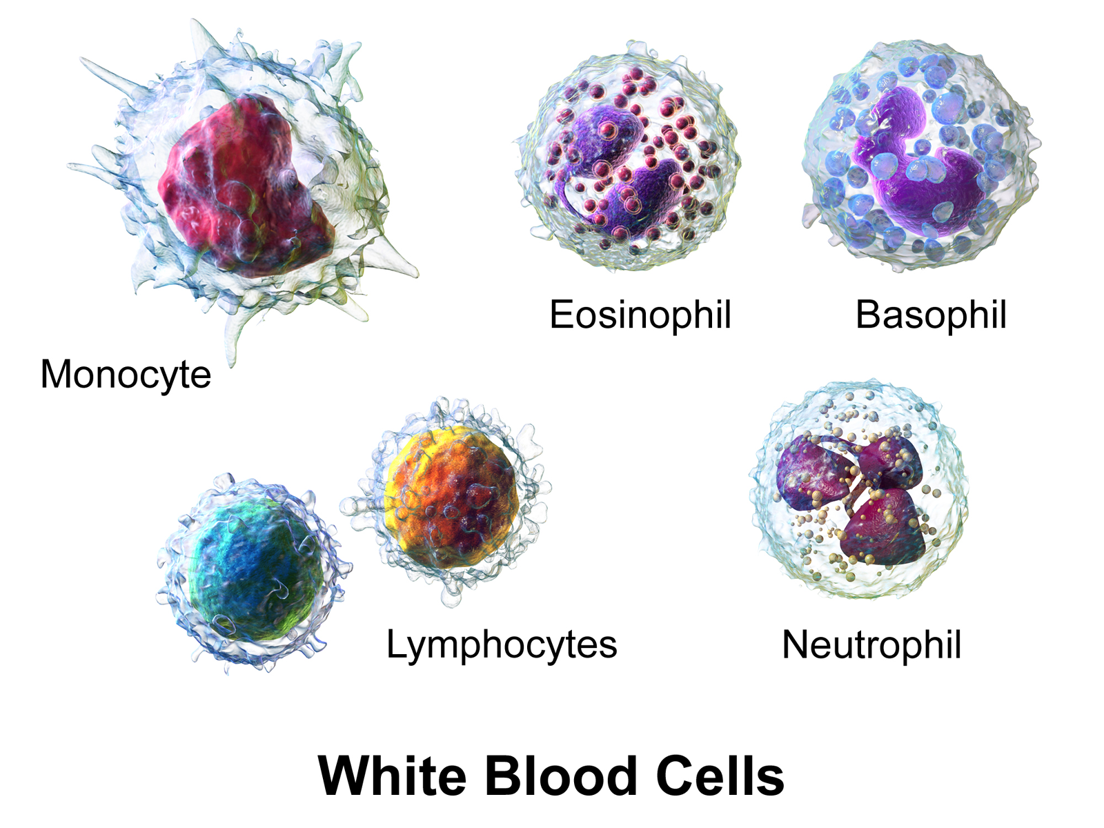
(Illustration from Wikipédia)

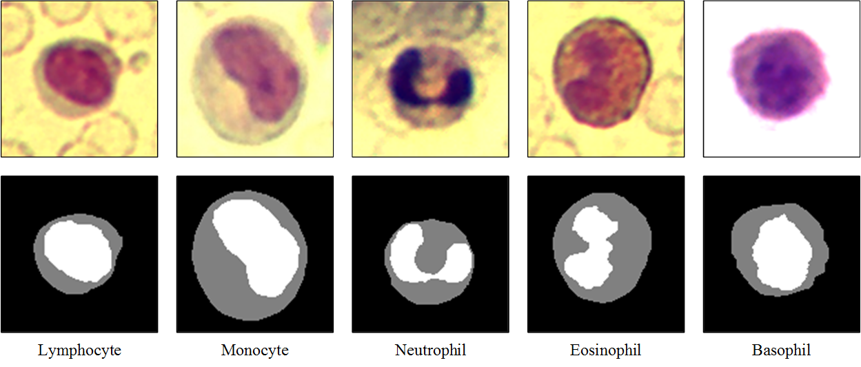
The dataset contains three hundred 120×120 RGB images with one blood cell per image, and corresponding segmentation masks. The segmentation mask was manually sketched by domain experts, with the background, cytoplasms and nuclei pixels labelled as 0, 1 and 2 respectively.

These images and masks are in the data/bloodcells_seg/ folder:

└── data
    └── bloodcells_seg
        ├── masks
        │   └── all
        └── images
            └── all

We want to use convolutional neural networks to do pixel-wise classification of these blood cell images into background / cytoplasm / nuclei.

Setup

Code

import random
from pathlib import Path
from typing import Optional, Callable

import numpy as np
import matplotlib.pyplot as plt
from matplotlib.colors import ListedColormap
import plotly.graph_objects as go
from PIL import Image
from IPython.display import display, clear_output

import torch
import torch.nn as nn
import torch.optim as optim
import torch.nn.functional as F
from torch.utils.data import Dataset, DataLoader, random_split
from torchvision import transforms

device = torch.device('cuda') if torch.cuda.is_available() else torch.device('cpu')
print(f"Using device: {device}")

Loading the data

We build a small paired dataset that reads RGB images from data/bloodcells_seg/images/all/ and grayscale masks from data/bloodcells_seg/masks/all/. The masks store class indices {0, 1, 2} directly, so we load them as long tensors.

Code

IMG_SIZE = 128
NUM_CLASSES = 3   # background, cytoplasm, nuclei
N_CHANNELS = 3    # RGB
BATCH_SIZE = 8
SEED = 909


class SegDataset(Dataset):
    """Paired image / mask dataset. Assumes filenames match after sorting."""
    def __init__(self, image_dir: str, mask_dir: str, img_size: int):
        self.image_paths = sorted(Path(image_dir).glob('*'))
        self.mask_paths  = sorted(Path(mask_dir).glob('*'))
        assert len(self.image_paths) == len(self.mask_paths), (
            f"Mismatched counts: {len(self.image_paths)} images vs "
            f"{len(self.mask_paths)} masks"
        )
        self.img_size = img_size
        self.image_tf = transforms.Compose([
            transforms.Resize((img_size, img_size)),
            transforms.ToTensor(),              # [0,1] RGB, (C,H,W)
        ])
        self.mask_resize = transforms.Resize(
            (img_size, img_size),
            interpolation=transforms.InterpolationMode.NEAREST,
        )

    def __len__(self):
        return len(self.image_paths)

    def __getitem__(self, idx):
        img = Image.open(self.image_paths[idx]).convert('RGB')
        mask = Image.open(self.mask_paths[idx]).convert('L')
        img = self.image_tf(img)
        mask = self.mask_resize(mask)
        mask = torch.as_tensor(np.array(mask), dtype=torch.long)  # (H, W)
        return img, mask


dataset = SegDataset(
    image_dir='data/bloodcells_seg/images/all',
    mask_dir='data/bloodcells_seg/masks/all',
    img_size=IMG_SIZE,
)

# Train / development split — equivalent to Keras validation_split=0.2
n_total = len(dataset)
n_dev = int(0.2 * n_total)
n_train = n_total - n_dev
train_dataset, dev_dataset = random_split(
    dataset, [n_train, n_dev],
    generator=torch.Generator().manual_seed(SEED),
)

train_loader = DataLoader(train_dataset, batch_size=BATCH_SIZE, shuffle=True,  num_workers=2)
dev_loader   = DataLoader(dev_dataset,   batch_size=BATCH_SIZE, shuffle=False, num_workers=2)

print(f"Total samples: {n_total}")
print(f"Training samples: {n_train}")
print(f"Development samples: {n_dev}")

Check that the loader delivers our data

Code

cMap = ListedColormap(['red', 'lime', 'blue'])

images, masks = next(iter(train_loader))
for i in range(2):
    fig, (ax_img, ax_mask) = plt.subplots(1, 2, figsize=(8, 4))
    ax_img.imshow(images[i].permute(1, 2, 0).numpy())
    ax_img.set_title('Image')
    ax_img.axis('off')
    ax_mask.imshow(masks[i].numpy(), cmap=cMap, vmin=0, vmax=2)
    ax_mask.set_title('Mask')
    ax_mask.axis('off')
    plt.show()

Live plot

This cell defines a simple live plot used to follow the training and development losses in real time (same LivePlot class as in the classification lab).

Code

from plotly.subplots import make_subplots


class LivePlot():
    def __init__(self, prediction_rows=None,
                 prediction_name: str = "Development predictions"):
        self.fig = go.FigureWidget()
        self.plot_indices = {}
        display(self.fig)
        self.limits = [0, 0]
        self.current_x = 0
        self.grid_figs = {}
        if prediction_rows is not None:
            self.report_prediction_grid(prediction_name, prediction_rows)

    def report(self, name: str, value: float):
        try:
            plot_index = self.plot_indices[name]
        except KeyError:
            plot_index = len(self.fig.data)
            self.fig.add_scatter(y=[], x=[], name=name)
            self.plot_indices[name] = plot_index
        self.fig.data[plot_index].y += (value,)
        self.fig.data[plot_index].x += (self.current_x,)

    def report_prediction_grid(self, name: str, rows):
        """Display rows of (image, truth, prediction) and update in place.

        `rows` is a list of dicts: `{'image': (H,W,3) uint8, 'truth': (H,W) int,
        'pred': (H,W) int}`. On first call a subplot grid is created; on
        subsequent calls the trace data is replaced in place.
        """
        n_rows = len(rows)
        mask_colorscale = [[0.0, 'red'], [0.5, 'lime'], [1.0, 'blue']]
        if name not in self.grid_figs:
            fig = make_subplots(
                rows=n_rows, cols=3,
                column_titles=['Input', 'Ground truth', 'Prediction'],
                horizontal_spacing=0.02, vertical_spacing=0.04,
            )
            for i, row in enumerate(rows):
                fig.add_trace(go.Image(z=row['image']), row=i + 1, col=1)
                fig.add_trace(go.Heatmap(z=row['truth'], colorscale=mask_colorscale,
                                         zmin=0, zmax=2, showscale=False),
                              row=i + 1, col=2)
                fig.add_trace(go.Heatmap(z=row['pred'], colorscale=mask_colorscale,
                                         zmin=0, zmax=2, showscale=False),
                              row=i + 1, col=3)
            for r in range(1, n_rows + 1):
                for c in range(1, 4):
                    idx = 3 * (r - 1) + c
                    suffix = '' if idx == 1 else str(idx)
                    fig.layout[f'xaxis{suffix}'].update(showticklabels=False)
                    fig.layout[f'yaxis{suffix}'].update(
                        autorange='reversed', showticklabels=False,
                        scaleanchor=f'x{suffix}', scaleratio=1,
                    )
            fig.update_layout(height=250 * n_rows, width=800,
                              margin=dict(l=20, r=20, t=40, b=20),
                              title=name, showlegend=False)
            widget = go.FigureWidget(fig)
            display(widget)
            self.grid_figs[name] = widget
        else:
            widget = self.grid_figs[name]
            with widget.batch_update():
                for i, row in enumerate(rows):
                    widget.data[3 * i + 0].z = row['image']
                    widget.data[3 * i + 1].z = row['truth']
                    widget.data[3 * i + 2].z = row['pred']

    def increment(self, n_ticks: int):
        self.limits[1] += n_ticks
        self.fig.update_layout(xaxis_range=self.limits)

    def set_limit(self, n_ticks: int):
        self.limits[1] = n_ticks
        self.fig.update_layout(xaxis_range=self.limits)

    def tick(self, n_ticks: Optional[int] = None):
        if n_ticks is None:
            n_ticks = 1
        self.current_x += n_ticks

Predictions panel

After each epoch we refresh a live grid of (input, ground truth, prediction) rows for a few development examples, so we can follow the training of our network visually. We run it on a fixed batch so the same cells are tracked across epochs.

The helper below turns one batch (images, masks) into a list of rows ready for LivePlot.report_prediction_grid.

Code

def build_prediction_rows(model, batch, device, num_plot: int):
    images, masks = batch
    model.eval()
    with torch.no_grad():
        preds = model(images.to(device)).argmax(dim=1).cpu().numpy()
    k = min(num_plot, images.size(0))
    rows = []
    for i in range(k):
        img = (images[i].permute(1, 2, 0).numpy() * 255).clip(0, 255).astype(np.uint8)
        rows.append({
            'image': img,
            'truth': masks[i].numpy().astype(np.int32),
            'pred':  preds[i].astype(np.int32),
        })
    return rows

Training loop

Boilerplate training loop. It reports training/development loss after each epoch via LivePlot, and if a plot_batch is supplied it draws the predictions panel for that fixed batch each epoch.

Code

def train(*,
          model: nn.Module,
          train_loader: DataLoader,
          dev_loader: DataLoader,
          optimizer: torch.optim.Optimizer,
          criterion: nn.Module,
          max_epochs: int,
          device: Optional[torch.device] = None,
          liveplot: Optional[LivePlot] = None,
          plot_batch=None,
          num_plot: int = 2):
    if device is None:
        device = torch.device('cuda') if torch.cuda.is_available() else torch.device('cpu')
    model.to(device)

    for epoch in range(max_epochs):
        model.train()
        train_loss_acc = 0
        train_examples = 0
        for x_batch, y_batch in train_loader:
            optimizer.zero_grad()
            x_batch = x_batch.to(device)
            y_hat = model(x_batch)
            loss = criterion(y_hat, y_batch.to(device))
            loss.backward()
            optimizer.step()
            train_loss_acc += loss.item() * x_batch.size(0)
            train_examples += x_batch.size(0)

        model.eval()
        dev_loss_acc = 0
        dev_examples = 0
        with torch.no_grad():
            for x_batch, y_batch in dev_loader:
                x_batch = x_batch.to(device)
                y_hat = model(x_batch)
                dev_loss_acc += criterion(y_hat, y_batch.to(device)).item() * x_batch.size(0)
                dev_examples += x_batch.size(0)

        if liveplot is not None:
            liveplot.tick()
            liveplot.report("Training loss",   train_loss_acc / train_examples)
            liveplot.report("Development loss", dev_loss_acc   / dev_examples)

        if plot_batch is not None and liveplot is not None:
            rows = build_prediction_rows(model, plot_batch, device, num_plot)
            liveplot.report_prediction_grid("Development predictions", rows)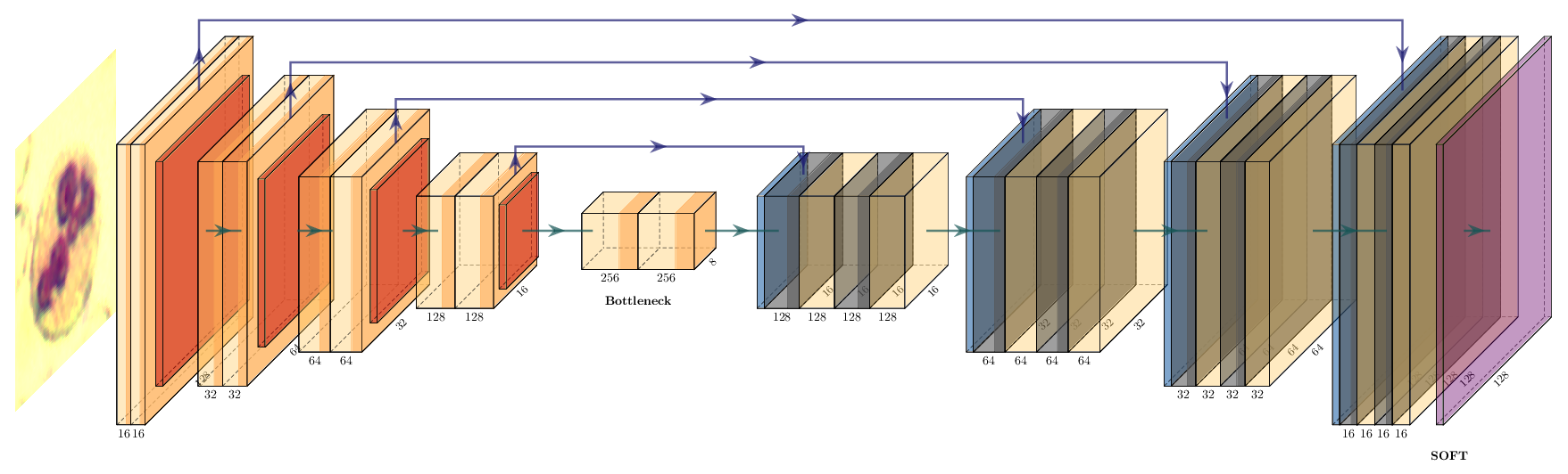

Building a U-Net model

In PyTorch we build the same architecture as a subclass of nn.Module. Each encoder / decoder block is two 3×3 convolutions (with same padding) and an ELU activation, with dropout between the two convolutions.

We use the ELU activation function: the negative values and the smooth transition from negative to positive help us converge faster in a low number of epochs. You can easily try other activations by replacing nn.ELU() with nn.ReLU(), nn.LeakyReLU(), etc.

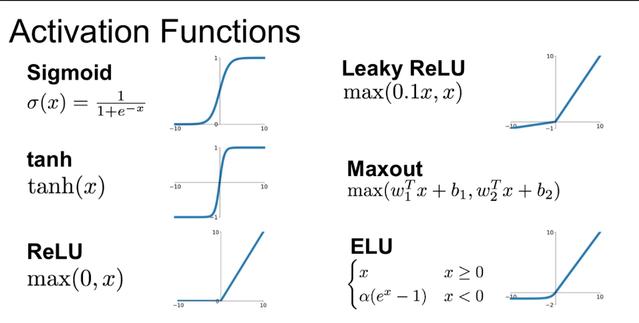
You can visualize differences between activation functions with this online tool from Justin Emery:

Code

from IPython.display import IFrame
IFrame('https://polarisation.github.io/tfjs-activation-functions/', width=860, height=470)

The U-Net architecture

Code

class ConvBlock(nn.Module):
    """Two 3×3 'same' convolutions with ELU and dropout in between."""
    def __init__(self, in_channels: int, out_channels: int, dropout: float):
        super().__init__()
        self.block = nn.Sequential(
            nn.Conv2d(in_channels, out_channels, kernel_size=3, padding=1),
            nn.ELU(inplace=True),
            nn.Dropout2d(dropout),
            nn.Conv2d(out_channels, out_channels, kernel_size=3, padding=1),
            nn.ELU(inplace=True),
        )

    def forward(self, x):
        return self.block(x)


class UNet(nn.Module):
    def __init__(self, in_channels: int = N_CHANNELS, num_classes: int = NUM_CLASSES):
        super().__init__()
        # Encoder
        self.enc1 = ConvBlock(in_channels, 16,  0.1)
        self.enc2 = ConvBlock(16,          32,  0.1)
        self.enc3 = ConvBlock(32,          64,  0.2)
        self.enc4 = ConvBlock(64,          128, 0.2)
        self.bottleneck = ConvBlock(128, 256, 0.3)
        self.pool = nn.MaxPool2d(2)
        # Decoder
        self.up4  = nn.ConvTranspose2d(256, 128, kernel_size=2, stride=2)
        self.dec4 = ConvBlock(256, 128, 0.2)
        self.up3  = nn.ConvTranspose2d(128, 64, kernel_size=2, stride=2)
        self.dec3 = ConvBlock(128, 64,  0.2)
        self.up2  = nn.ConvTranspose2d(64,  32, kernel_size=2, stride=2)
        self.dec2 = ConvBlock(64,  32,  0.1)
        self.up1  = nn.ConvTranspose2d(32,  16, kernel_size=2, stride=2)
        self.dec1 = ConvBlock(32,  16,  0.1)
        # Pixel-wise classifier
        self.out_conv = nn.Conv2d(16, num_classes, kernel_size=1)

        # He-normal init to match Keras `kernel_initializer='he_normal'`
        for m in self.modules():
            if isinstance(m, (nn.Conv2d, nn.ConvTranspose2d)):
                nn.init.kaiming_normal_(m.weight, nonlinearity='relu')
                if m.bias is not None:
                    nn.init.zeros_(m.bias)

    def forward(self, x):
        c1 = self.enc1(x)
        c2 = self.enc2(self.pool(c1))
        c3 = self.enc3(self.pool(c2))
        c4 = self.enc4(self.pool(c3))
        c5 = self.bottleneck(self.pool(c4))

        d4 = self.dec4(torch.cat([self.up4(c5), c4], dim=1))
        d3 = self.dec3(torch.cat([self.up3(d4), c3], dim=1))
        d2 = self.dec2(torch.cat([self.up2(d3), c2], dim=1))
        d1 = self.dec1(torch.cat([self.up1(d2), c1], dim=1))
        return self.out_conv(d1)  # logits, shape (N, num_classes, H, W)


model = UNet().to(device)
print(model)
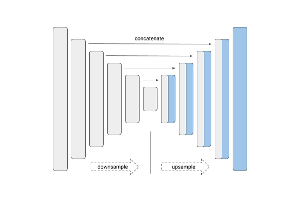
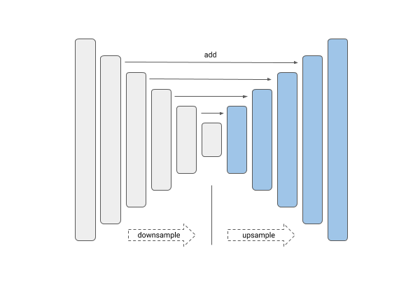
print(f"Total parameters: {sum(p.numel() for p in model.parameters()):,}")

As our ground truth is represented by integer class indices on the mask (0 / 1 / 2) and not one-hot encoded, we use nn.CrossEntropyLoss, which applies log_softmax internally and expects raw logits — the PyTorch equivalent of SparseCategoricalCrossentropy(from_logits=False).

Code

criterion = nn.CrossEntropyLoss()
optimizer = optim.Adam(model.parameters(), lr=1e-4)

Train the model

We pick a fixed development batch so the predictions panel tracks the same cells across epochs.

Code

plot_batch = next(iter(dev_loader))
initial_rows = build_prediction_rows(model, plot_batch, device, num_plot=3)
liveplot = LivePlot(prediction_rows=initial_rows)

Code

epochs = 20
liveplot.increment(epochs)
train(model=model, train_loader=train_loader, dev_loader=dev_loader,
      optimizer=optimizer, criterion=criterion, max_epochs=epochs,
      device=device, liveplot=liveplot,
      plot_batch=plot_batch, num_plot=3)

More development examples

Code

rows = build_prediction_rows(model, next(iter(dev_loader)), device, BATCH_SIZE)
liveplot.report_prediction_grid("Final predictions", rows)

Tuning of the model

You can now try to tune your model by changing the learning rate of the Adam optimizer, the dropout, the batch size, or any other parameter you want.

Other models

To simplify the construction of our networks, we can use the segmentation_models_pytorch library (the PyTorch equivalent of the segmentation_models library used in the Keras lab). Install it with:

pip install segmentation_models_pytorch

The main features of this library are:

High-level API (just two lines of code to create a segmentation model)
Several model architectures for binary and multi-class image segmentation (including U-Net, Linknet, FPN, PSPNet, DeepLabV3+, …)
Dozens of pre-defined encoders (backbones) for each architecture

List of models:

Unet	Linknet

PSPNet	FPN

List of backbones (encoders):

Type	Names
VGG	`vgg11` `vgg13` `vgg16` `vgg19`
ResNet	`resnet18` `resnet34` `resnet50` `resnet101` `resnet152`
SE-ResNet	`se_resnet50` `se_resnet101` `se_resnet152`
ResNeXt	`resnext50_32x4d` `resnext101_32x8d`
SE-ResNeXt	`se_resnext50_32x4d` `se_resnext101_32x4d`
SENet154	`senet154`
DenseNet	`densenet121` `densenet169` `densenet201`
Inception	`inceptionv4` `inceptionresnetv2`
MobileNet	`mobilenet_v2`
EfficientNet	`efficientnet-b0` … `efficientnet-b7`

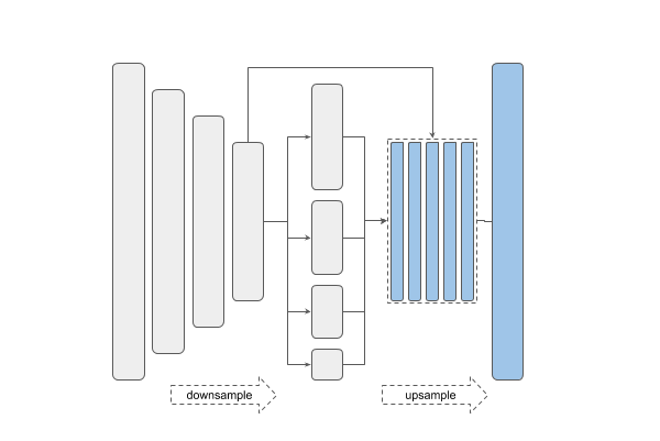
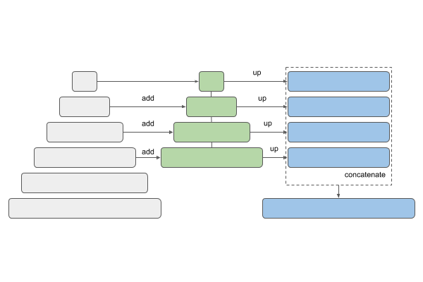
U-Net and Link-Net are similar and generally used for the kind of segmentation we have here. FPN (Feature Pyramid Networks) are mainly used for object detection, and PSPNet (Pyramid Scene Parsing Networks) are another family of segmentation models — see this overview.

Code

import segmentation_models_pytorch as smp

# Load a U-Net with a VGG16 backbone, trained from scratch
model = smp.Unet(
    encoder_name='vgg16',
    encoder_weights="imagenet",
    in_channels=N_CHANNELS,
    classes=NUM_CLASSES,
).to(device)

print(model)
print(f"Total parameters: {sum(p.numel() for p in model.parameters()):,}")

Compile and train with the same parameters as before

Code

criterion = nn.CrossEntropyLoss()
optimizer = optim.Adam(model.parameters(), lr=1e-4)

initial_rows = build_prediction_rows(model, plot_batch, device, num_plot=2)
liveplot = LivePlot(prediction_rows=initial_rows)

Code

epochs = 30
liveplot.increment(epochs)
train(model=model, train_loader=train_loader, dev_loader=dev_loader,
      optimizer=optimizer, criterion=criterion, max_epochs=epochs,
      device=device, liveplot=liveplot,
      plot_batch=plot_batch, num_plot=2)

Code

rows = build_prediction_rows(model, next(iter(dev_loader)), device, BATCH_SIZE)
liveplot.report_prediction_grid("Final predictions (smp U-Net / VGG16)", rows)