CNN Lab 1: Classification of Human Blood Cells using PyTorch

Classify human blood cell images with PyTorch, progressing from a minimal CNN to an advanced CNN and finally to VGG16.

Author

Affiliation

Christophe Avenel

NBIS

Running on colab

To run this notebook on Google Colab:

Download the notebook from this link.
Go to colab.research.google.com, then File → Open notebook → Upload and select the downloaded file.
Make a copy to your own Google Drive before starting your work, so that your changes are saved.
Download and unzip the data by running the following in a new cell:

Code

!wget https://user.it.uu.se/~chrav452/workshop_NN_DL_cnn_data.zip
!unzip workshop_NN_DL_cnn_data.zip

Classification of Human Blood Cells using Convolutional Neural Networks

For this lab, we use the image set Human White Blood Cells (BBBC045v1) from the Broad Bioimage Benchmark Collection [Ljosa et al., Nature Methods, 2012].

Using fluorescence staining (Label‐Free Identification of White Blood Cells Using Machine Learning (Nassar et. al)), each blood cell has been classified into one of 5 categories:

B cells (lymphocytes)
T cells (lymphocytes)
eosinophils
monocytes
neutrophils

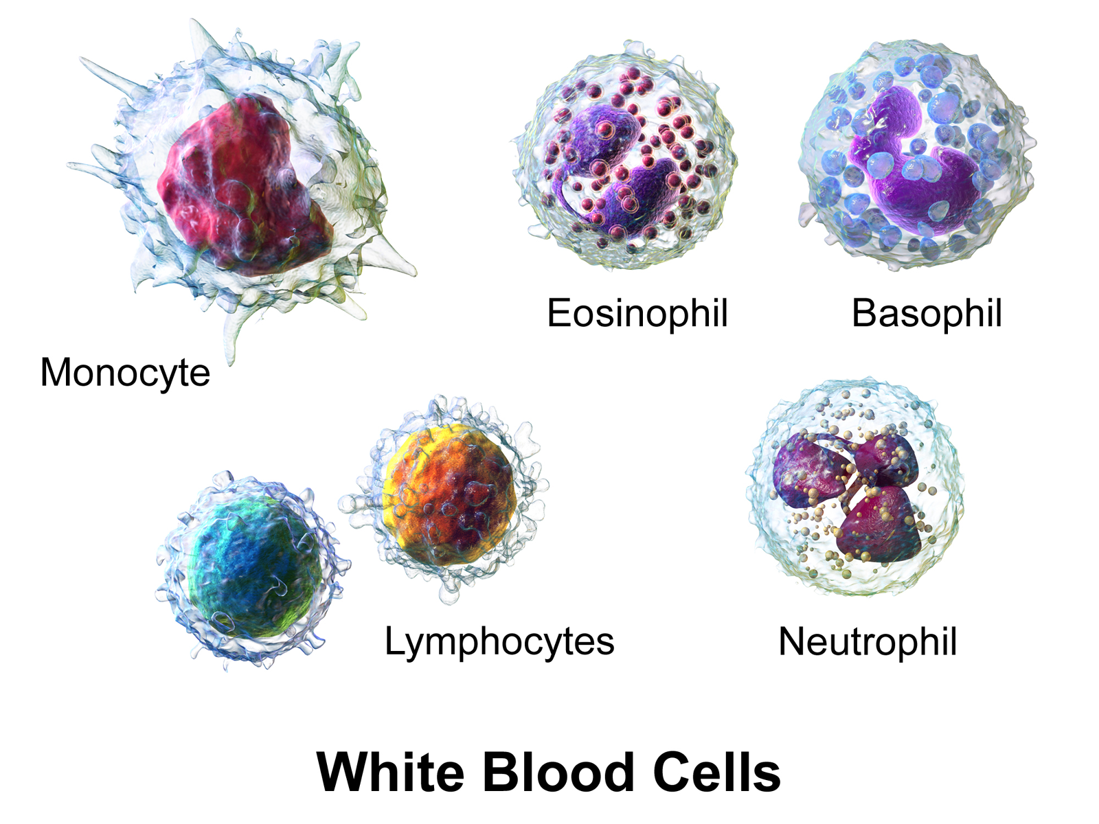
(Illustration from Wikipédia)

Brightfield dataset

For this lab, we only kept Brightfield images and cropped them into small grayscale patches of 32×32 pixels:

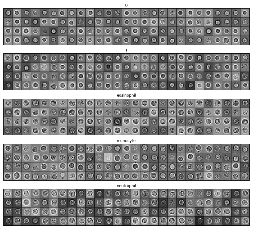
These patches are in the data/bloodcells_small/ folder, split into testing and training sets. In each set, images are split according to their categories:

└── data
    └── bloodcells_small
        ├── test
        │   ├── B
        │   ├── T
        │   ├── eosinophil
        │   ├── monocyte
        │   └── neutrophil
        └── train
            ├── B
            ├── T
            ├── eosinophil
            ├── monocyte
            └── neutrophil

Our goal is to use convolutional neural networks to automatically classify blood cells into one of the five categories, using only the 32×32 pixels brightfield images.

Setup

Code

import random
import itertools
from typing import Optional
from collections import Counter

import numpy as np
import matplotlib.pyplot as plt
import plotly.graph_objects as go

import torch
import torch.nn as nn
import torch.optim as optim
from torch.utils.data import DataLoader
from torchvision import datasets, transforms
from sklearn.metrics import confusion_matrix

# Check for GPU
device = torch.device('cuda') if torch.cuda.is_available() else torch.device('cpu')
print(f"Using device: {device}")

Loading the data

We use ImageFolder and DataLoader to create loaders for the training and testing datasets. ImageFolder reads the class of each image from the directory structure.

We also match the per-sample centering / standardization from the original Keras notebook (samplewise_center=True, samplewise_std_normalization=True) with a small custom transform.

Code

IMG_SIZE = 32
BATCH_SIZE = 8
NUM_CLASSES = 5


def samplewise_standardize(x: torch.Tensor) -> torch.Tensor:
    """Zero-mean, unit-std per image (matches Keras `samplewise_*` flags)."""
    return (x - x.mean()) / (x.std() + 1e-6)


gray_transform = transforms.Compose([
    transforms.Grayscale(),
    transforms.Resize((IMG_SIZE, IMG_SIZE)),
    transforms.ToTensor(),          # [0,1], (C,H,W)
    transforms.Lambda(samplewise_standardize),
])

train_dataset = datasets.ImageFolder('data/bloodcells_small/train/', transform=gray_transform)
dev_dataset   = datasets.ImageFolder('data/bloodcells_small/test/',  transform=gray_transform)

train_loader = DataLoader(train_dataset, batch_size=BATCH_SIZE, shuffle=True,  num_workers=2)
dev_loader   = DataLoader(dev_dataset,   batch_size=BATCH_SIZE, shuffle=False, num_workers=2)

print(f"Classes: {train_dataset.classes}")
print(f"Class to index mapping: {train_dataset.class_to_idx}")
print(f"Training samples: {len(train_dataset)}")
print(f"Testing samples:  {len(dev_dataset)}")

Images per class

Code

def class_sizes(dataset):
    return dict(Counter(dataset.classes[t] for _, t in dataset.samples))

print("Images per class in training:", class_sizes(train_dataset))
print("Images per class in testing: ", class_sizes(dev_dataset))

Check that the loader delivers our data

Code

num_images = 5
for i in range(num_images):
    idx = random.randrange(len(train_dataset))
    image, label = train_dataset[idx]
    img = image.squeeze().numpy()  # (H, W) for grayscale display

    print(f"Category: {train_dataset.classes[label]} (index={label})")
    print(f"Image shape: {img.shape}")
    plt.imshow(img, cmap='gray')
    plt.axis('off')
    plt.show()

Live plot

This cell defines a simple live plot used to follow the training loss, the development loss, and the development confusion matrix in real time.

Code

class LivePlot():
    def __init__(self):
        self.fig = go.FigureWidget()
        self.plot_indices = {}
        display(self.fig)
        self.limits = [0, 0]
        self.current_x = 0
        self.matrix_figs = {}

    def report(self, name: str, value: float):
        "Report new value for line `name` of the current time step."
        try:
            plot_index = self.plot_indices[name]
        except KeyError:
            plot_index = len(self.fig.data)
            self.fig.add_scatter(y=[], x=[], name=name)
            self.plot_indices[name] = plot_index
        self.fig.data[plot_index].y += (value,)
        self.fig.data[plot_index].x += (self.current_x,)

    def report_matrix(self, name: str, matrix, labels=None):
        "Replace the heatmap `name` with `matrix`. Creates a new figure on first call."
        matrix = np.asarray(matrix)
        n_rows, n_cols = matrix.shape
        x_labels = list(labels) if labels is not None else list(range(n_cols))
        y_labels = list(labels) if labels is not None else list(range(n_rows))
        thresh = float(matrix.max()) / 2.
        annotations = [
            dict(x=x_labels[j], y=y_labels[i],
                 text=f"{100*matrix[i, j]:.0f}%",
                 showarrow=False,
                 font=dict(color="white" if matrix[i, j] > thresh else "black"))
            for i in range(n_rows) for j in range(n_cols)
        ]
        if name not in self.matrix_figs:
            fig = go.FigureWidget(
                data=[go.Heatmap(z=matrix, x=x_labels, y=y_labels,
                                 colorscale='Blues', zmin=0, zmax=1)]
            )
            fig.update_layout(
                title=name,
                xaxis=dict(title='Predicted label', constrain='domain'),
                yaxis=dict(title='True label', autorange='reversed',
                           scaleanchor='x', scaleratio=1),
                width=600, height=600,
                annotations=annotations,
            )
            display(fig)
            self.matrix_figs[name] = fig
        else:
            fig = self.matrix_figs[name]
            fig.data[0].z = matrix
            fig.layout.annotations = annotations

    def increment(self, n_ticks: int):
        "Increment the currently displayed limits with these many ticks."
        self.limits[1] += n_ticks
        self.fig.update_layout(xaxis_range=self.limits)

    def set_limit(self, n_ticks: int):
        "Update the currently displayed to exactly these many ticks."
        self.limits[1] = n_ticks
        self.fig.update_layout(xaxis_range=self.limits)

    def tick(self, n_ticks: Optional[int] = None):
        "Update the current time with these many ticks, or 1 tick if omitted."
        if n_ticks is None:
            n_ticks = 1
        self.current_x += n_ticks

Training loop

Boilerplate training loop. It runs max_epochs epochs, reports the training and development loss after each epoch, and (if a LivePlot is supplied) updates a live confusion matrix on the development set.

Code

def train(*,
          model: nn.Module,
          train_loader: DataLoader,
          dev_loader: DataLoader,
          optimizer: torch.optim.Optimizer,
          criterion: nn.Module,
          max_epochs: int,
          device: Optional[torch.device] = None,
          liveplot: Optional[LivePlot] = None):
    if device is None:
        device = torch.device('cuda') if torch.cuda.is_available() else torch.device('cpu')

    model.to(device)

    for epoch in range(max_epochs):
        training_loss_acc = 0
        training_examples = 0
        model.train()

        for x_batch, y_batch in train_loader:
            optimizer.zero_grad()
            x_batch = x_batch.to(device)
            y_hat = model(x_batch)
            loss = criterion(y_hat, y_batch.to(device))
            loss.backward()
            optimizer.step()
            training_loss_acc += loss.item()
            training_examples += x_batch.size(0)

        model.eval()
        dev_preds, dev_labels = [], []
        with torch.no_grad():
            dev_loss_acc = 0
            dev_examples = 0
            for x_batch, y_batch in dev_loader:
                x_batch = x_batch.to(device)
                y_hat = model(x_batch)
                dev_loss_acc += criterion(y_hat, y_batch.to(device)).item()
                dev_examples += x_batch.size(0)
                dev_preds.append(y_hat.argmax(1).cpu().numpy())
                dev_labels.append(y_batch.numpy())

        if liveplot is not None:
            liveplot.tick()
            liveplot.report("Training loss", training_loss_acc / training_examples)
            liveplot.report("Development loss", dev_loss_acc / dev_examples)

            y_pred = np.concatenate(dev_preds)
            y_true = np.concatenate(dev_labels)
            n_classes = int(max(y_true.max(), y_pred.max())) + 1
            cm = confusion_matrix(y_true, y_pred, labels=list(range(n_classes)))
            cm_norm = cm.astype('float') / cm.sum(axis=1, keepdims=True).clip(min=1)
            class_names = getattr(dev_loader.dataset, 'classes', None)
            liveplot.report_matrix("Confusion matrix (dev)", cm_norm, labels=class_names)

Training the model

A first CNN model

We can start by building a simple convolutional network with one convolutional layer followed by one max-pooling layer.

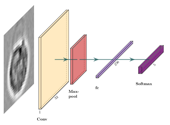
The equivalent in PyTorch is a subclass of nn.Module:

Code

class SimpleCNN(nn.Module):
    """1 conv layer + 1 max-pool + 1 fully connected layer."""
    def __init__(self, num_classes=NUM_CLASSES):
        super().__init__()
        num_filters = 1
        filter_size = 2
        pool_size = 2
        # Conv with 'valid' padding: 32 - 2 + 1 = 31, then pool/2 -> 15
        self.conv = nn.Conv2d(1, num_filters, kernel_size=filter_size)
        self.pool = nn.MaxPool2d(pool_size)
        self.flatten = nn.Flatten()
        self.fc = nn.Linear(num_filters * 15 * 15, num_classes)

    def forward(self, x):
        x = self.conv(x)
        x = self.pool(x)
        x = self.flatten(x)
        return self.fc(x)  # logits — CrossEntropyLoss applies softmax internally


model = SimpleCNN().to(device)
print(model)
print(f"Total parameters: {sum(p.numel() for p in model.parameters()):,}")

criterion = nn.CrossEntropyLoss()
optimizer = optim.Adam(model.parameters())

Train the model on our data

We create a fresh LivePlot each time we train a new model so we can keep the history of each run around.

Code

liveplot = LivePlot()

Code

epochs = 5
liveplot.increment(epochs)
train(model=model, train_loader=train_loader, dev_loader=dev_loader,
      optimizer=optimizer, criterion=criterion, max_epochs=epochs,
      device=device, liveplot=liveplot)

Predictions on a random batch

Code

dev_iter = iter(DataLoader(dev_dataset, batch_size=BATCH_SIZE, shuffle=True))
images, labels = next(dev_iter)
model.eval()
with torch.no_grad():
    logits = model(images.to(device))
    predictions = logits.argmax(1).cpu().numpy()

print("Predictions:   ", predictions)
print("Ground truth:  ", labels.numpy())

Extensions

We can now modify our network to improve the accuracy of our classification.

Network depth

You can add more convolutional and max-pooling layers, and change the number of features in each convolutional layer. For example, two iterations of convolutional layer plus max-pooling, with 16 and 32 features and a kernel size of 3:

nn.Sequential(
    nn.Conv2d(1, 16, kernel_size=3),
    nn.MaxPool2d(2),
    nn.Conv2d(16, 32, kernel_size=3),
    nn.MaxPool2d(2),
    # ...
)

Dropout

Dropout layers can prevent overfitting. You can add dropout after max-pooling. A dropout of 20% is a good starting point.

nn.Dropout(0.2)

Fully-connected layers

Most CNNs use multiple fully-connected layers before the final classifier:

nn.Linear(in_features, 64),
nn.ReLU(),

Convolution parameters

Try adding an activation after convolutional layers (nn.ReLU()), and play with stride and padding (docs):

nn.Conv2d(in_channels, out_channels, kernel_size, stride=2, padding=1)

Learning rate

You can change the learning rate of the Adam optimizer:

optimizer = optim.Adam(model.parameters(), lr=1e-4)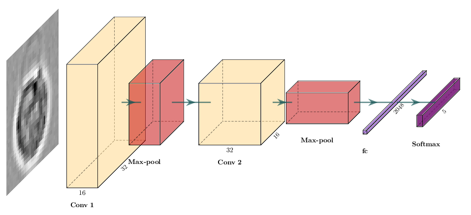

Example of a more advanced convolutional neural network:

Here we build that model with nn.Sequential, which is a concise alternative to subclassing nn.Module:

Code

num_filters = 16
# After conv(3, valid) + pool(2) twice on a 32x32 input: 32->30->15->13->6
flatten_features = (num_filters * 2) * 6 * 6

model = nn.Sequential(
    nn.Conv2d(1, num_filters, kernel_size=3),
    nn.ReLU(),
    nn.BatchNorm2d(num_filters),
    nn.MaxPool2d(2),
    nn.Dropout(0.2),

    nn.Conv2d(num_filters, num_filters * 2, kernel_size=3),
    nn.ReLU(),
    nn.MaxPool2d(2),
    nn.Dropout(0.2),

    nn.Flatten(),
    nn.Linear(flatten_features, num_filters * 8),
    nn.ReLU(),
    nn.Linear(num_filters * 8, NUM_CLASSES),
).to(device)

print(model)
print(f"Total parameters: {sum(p.numel() for p in model.parameters()):,}")

criterion = nn.CrossEntropyLoss()
optimizer = optim.Adam(model.parameters(), lr=1e-4)

Train the model

Code

liveplot = LivePlot()

Code

epochs = 5
liveplot.increment(epochs)
train(model=model, train_loader=train_loader, dev_loader=dev_loader,
      optimizer=optimizer, criterion=criterion, max_epochs=epochs,
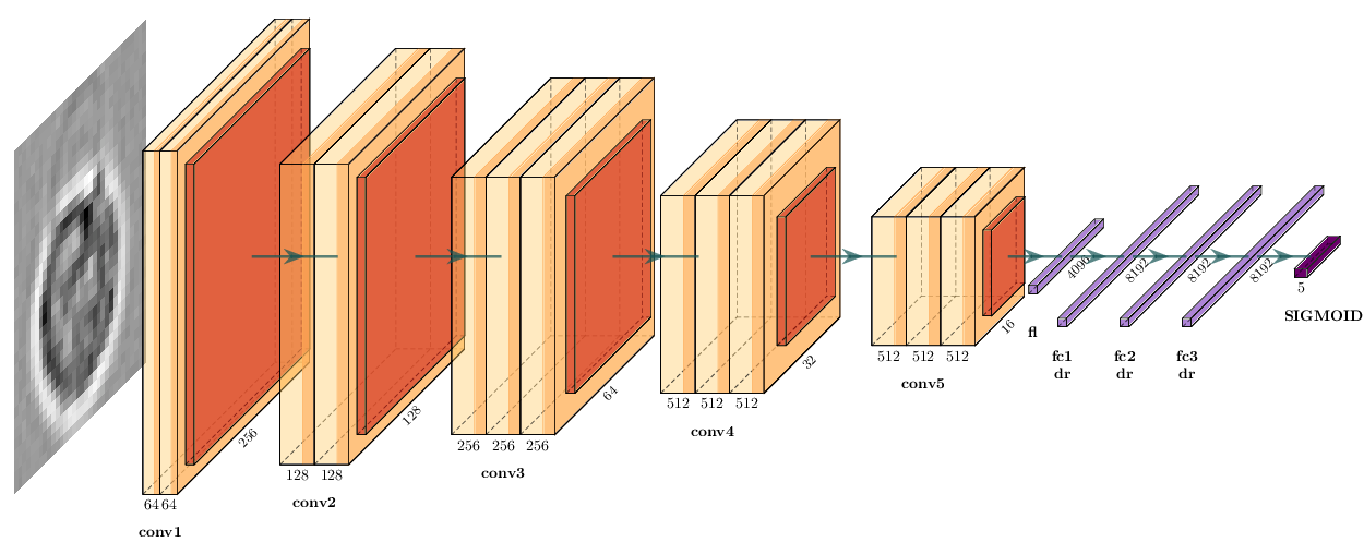
      device=device, liveplot=liveplot)

Example of a VGG16 network

VGG16 is a Convolutional Neural Network with five convolutional blocks followed by three fully-connected layers:

We need to load the data in RGB color mode, as VGG16 expects input with 3 channels:

Code

rgb_transform = transforms.Compose([
    transforms.Resize((IMG_SIZE, IMG_SIZE)),
    transforms.ToTensor(),
    transforms.Lambda(samplewise_standardize),
])

rgb_train = datasets.ImageFolder('data/bloodcells_small/train/', transform=rgb_transform)
rgb_dev   = datasets.ImageFolder('data/bloodcells_small/test/',  transform=rgb_transform)

rgb_train_loader = DataLoader(rgb_train, batch_size=BATCH_SIZE, shuffle=True,  num_workers=2)
rgb_dev_loader   = DataLoader(rgb_dev,   batch_size=BATCH_SIZE, shuffle=False, num_workers=2)

We load VGG16 from torchvision.models (with randomly initialized weights), drop its ImageNet classifier, and replace it with our own. With a 32×32 input, the five max-pool blocks reduce the feature map to 1×1, so we force the adaptive pooling layer to (1, 1) and feed a 512-dim vector into the new classifier head.

Code

from torchvision.models import vgg16

vgg = vgg16(weights=None)
vgg.avgpool = nn.AdaptiveAvgPool2d((1, 1))
vgg.classifier = nn.Sequential(
    nn.Flatten(),
    nn.Linear(512, 1024),
    nn.ReLU(),
    nn.Linear(1024, NUM_CLASSES),
)
vgg = vgg.to(device)

print(vgg)
print(f"Total parameters: {sum(p.numel() for p in vgg.parameters()):,}")

criterion = nn.CrossEntropyLoss()
optimizer = optim.Adam(vgg.parameters(), lr=1e-4)

Code

liveplot = LivePlot()

Code

epochs = 5
liveplot.increment(epochs)
train(model=vgg, train_loader=rgb_train_loader, dev_loader=rgb_dev_loader,
      optimizer=optimizer, criterion=criterion, max_epochs=epochs,
      device=device, liveplot=liveplot)