suppressPackageStartupMessages({
    library(scater)
    library(scran)
    # library(venn)
    library(patchwork)
    library(ggplot2)
    library(pheatmap)
    library(igraph)
    library(dplyr)
})
Note
Code chunks run R commands unless otherwise specified.
In this tutorial we will cover differential gene expression, which comprises an extensive range of topics and methods. In single cell, differential expresison can have multiple functionalities such as identifying marker genes for cell populations, as well as identifying differentially regulated genes across conditions (healthy vs control). We will also cover controlling batch effect in your test.
We can first load the data from the clustering session. Moreover, we can already decide which clustering resolution to use. First let’s define using the louvain clustering to identifying differentially expressed genes.
# download pre-computed data if missing or long compute
fetch_data <- TRUE

# url for source and intermediate data
path_data <- "https://export.uppmax.uu.se/naiss2023-23-3/workshops/workshop-scrnaseq"
path_file <- "data/covid/results/bioc_covid_qc_dr_int_cl.rds"
if (!dir.exists(dirname(path_file))) dir.create(dirname(path_file), recursive = TRUE)
if (fetch_data && !file.exists(path_file)) download.file(url = file.path(path_data, "covid/results/bioc_covid_qc_dr_int_cl.rds"), destfile = path_file)
sce <- readRDS(path_file)
print(reducedDims(sce))
List of length 16
names(16): PCA UMAP tSNE_on_PCA ... Scanorama_PCA UMAP_on_Scanorama SNN1 Cell marker genes
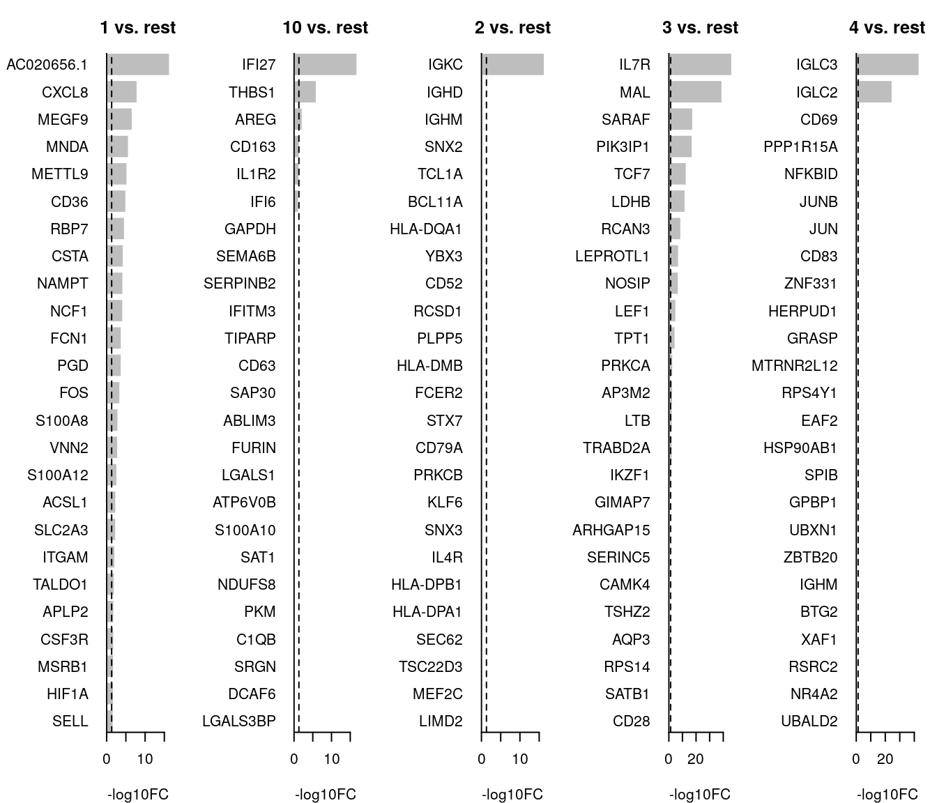
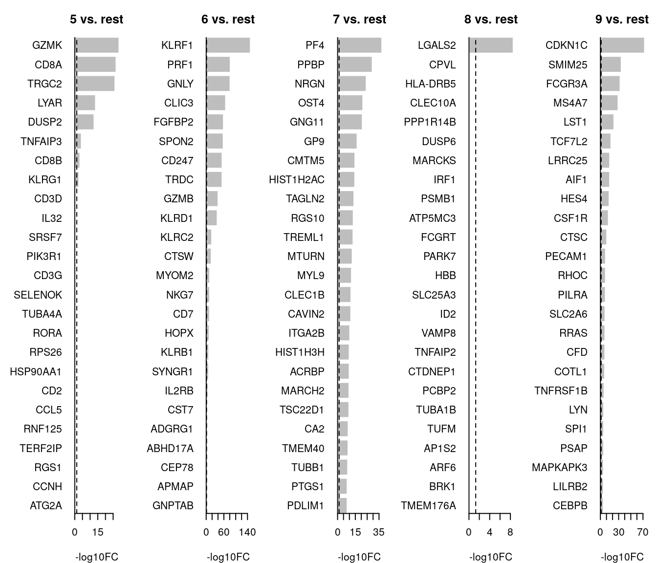
Let us first compute a ranking for the highly differential genes in each cluster. There are many different tests and parameters to be chosen that can be used to refine your results. When looking for marker genes, we want genes that are positively expressed in a cell type and possibly not expressed in others.
# Compute differentiall expression
markers_genes <- scran::findMarkers(
    x = sce,
    groups = as.character(sce$louvain_SNNk15),
    lfc = .5,
    pval.type = "all",
    direction = "up"
)

# List of dataFrames with the results for each cluster
markers_genes
List of length 10
names(10): 1 10 2 3 4 5 6 7 8 9# Visualizing the expression of one
markers_genes[["1"]]DataFrame with 18863 rows and 12 columns
p.value FDR summary.logFC logFC.10 logFC.2
<numeric> <numeric> <numeric> <numeric> <numeric>
AC020656.1 3.95594e-17 7.46208e-13 3.21182 3.21182 4.07138
CXCL8 1.08001e-08 1.01861e-04 1.17885 1.17885 1.20816
MEGF9 2.05097e-07 1.28958e-03 0.68677 1.18624 1.11914
MNDA 1.86611e-06 8.80009e-03 1.94630 1.94630 2.91834
METTL9 4.58358e-06 1.72920e-02 1.29770 1.29770 1.29491
... ... ... ... ... ...
AL354822.1 1 1 0.00148695 0.00148695 -0.01031833
AC004556.1 1 1 -0.01087034 0.00307313 -0.00110682
AC233755.2 1 1 0.00000000 0.00000000 0.00000000
AC233755.1 1 1 0.00000000 0.00000000 -0.01309954
AC240274.1 1 1 0.01348245 0.01348245 -0.00242453
logFC.3 logFC.4 logFC.5 logFC.6 logFC.7
<numeric> <numeric> <numeric> <numeric> <numeric>
AC020656.1 4.08487 4.06902 4.07511 4.06273 3.89033
CXCL8 1.29991 1.14612 1.24203 1.27109 1.10972
MEGF9 1.12684 1.14754 1.11072 1.06497 1.18624
MNDA 3.10873 2.92630 3.08248 3.11241 2.96624
METTL9 1.09055 1.25940 1.04031 1.12601 1.42409
... ... ... ... ... ...
AL354822.1 -0.00331466 -0.01067605 -0.008545897 -0.01865530 0.00148695
AC004556.1 -0.02752682 0.00921674 -0.041792826 -0.01087034 0.03772978
AC233755.2 0.00000000 -0.00525802 0.000000000 0.00000000 0.00000000
AC233755.1 0.00000000 -0.01266869 0.000000000 0.00000000 0.00000000
AC240274.1 -0.00497463 -0.00634737 0.000637567 0.00411926 -0.00882371
logFC.8 logFC.9
<numeric> <numeric>
AC020656.1 1.144302 3.10497
CXCL8 1.042347 1.26678
MEGF9 0.686770 0.80094
MNDA 1.220445 1.89668
METTL9 0.715494 1.07643
... ... ...
AL354822.1 -0.00148057 -0.0121590
AC004556.1 -0.07790786 -0.1310696
AC233755.2 0.00000000 0.0000000
AC233755.1 0.00000000 0.0000000
AC240274.1 -0.00622230 -0.0161392We can now select the top 25 overexpressed genes for plotting.
# Colect the top 25 genes for each cluster and put the into a single table
top25 <- lapply(names(markers_genes), function(x) {
    temp <- markers_genes[[x]][1:25, 1:2]
    temp$gene <- rownames(markers_genes[[x]])[1:25]
    temp$cluster <- x
    return(temp)
})
top25 <- as_tibble(do.call(rbind, top25))
top25$p.value[top25$p.value == 0] <- 1e-300
top25par(mfrow = c(1, 5), mar = c(4, 6, 3, 1))
for (i in unique(top25$cluster)) {
barplot(sort(setNames(-log10(top25$p.value), top25$gene)[top25$cluster == i], F),
horiz = T, las = 1, main = paste0(i, " vs. rest"), border = "white", yaxs = "i", xlab = "-log10FC"
)
abline(v = c(0, -log10(0.05)), lty = c(1, 2))
}
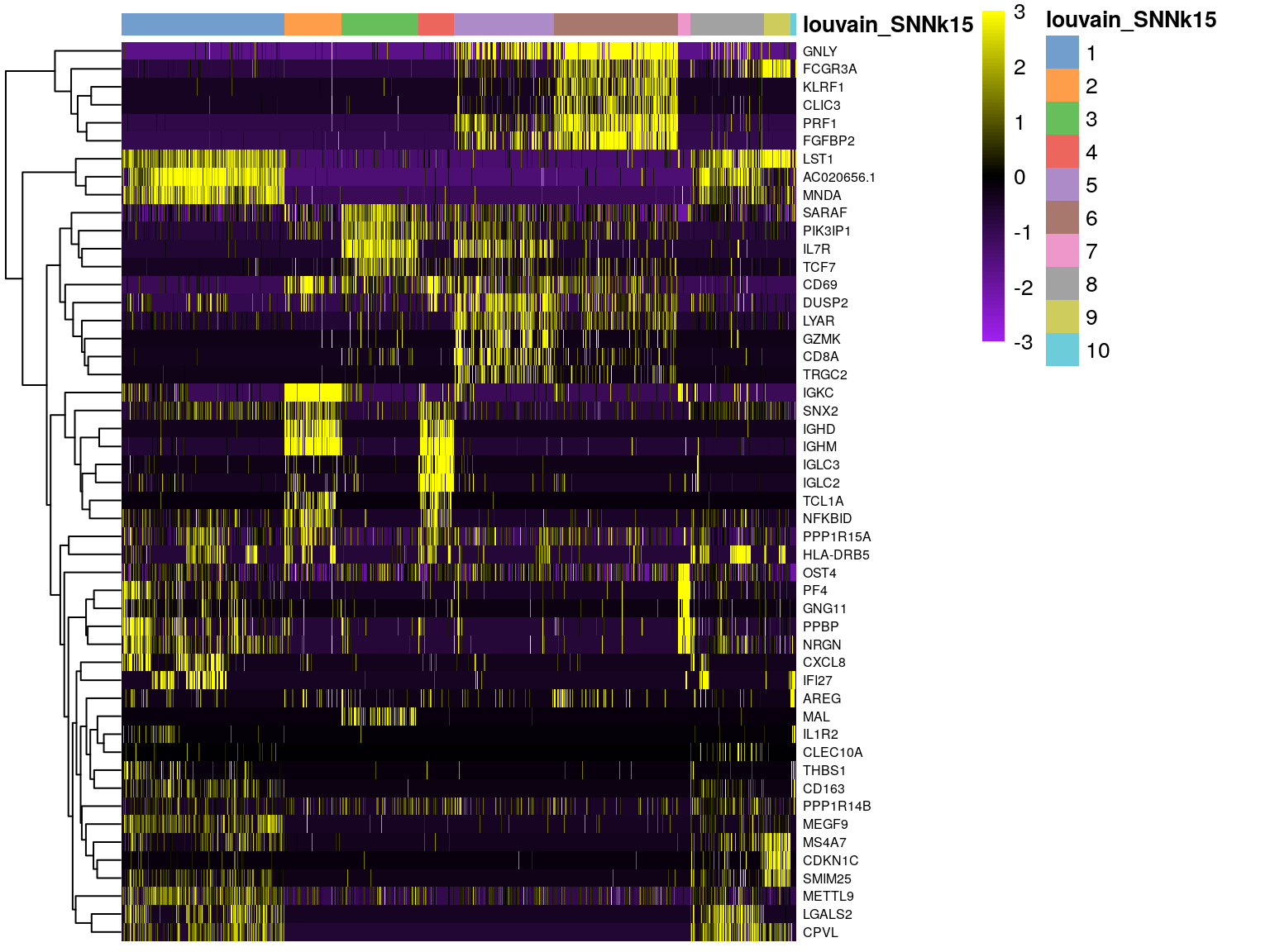
We can visualize them as a heatmap. Here we are selecting the top 5.
as_tibble(top25) %>%
    group_by(cluster) %>%
    top_n(-5, p.value) -> top5

scater::plotHeatmap(sce[, order(sce$louvain_SNNk15)],
    features = unique(top5$gene),
    center = T, zlim = c(-3, 3),
    colour_columns_by = "louvain_SNNk15",
    show_colnames = F, cluster_cols = F,
    fontsize_row = 6,
    color = colorRampPalette(c("purple", "black", "yellow"))(90)
)
We can also plot a violin plot for each gene.
scater::plotExpression(sce, features = unique(top5$gene), x = "louvain_SNNk15", ncol = 5, colour_by = "louvain_SNNk15", scales = "free")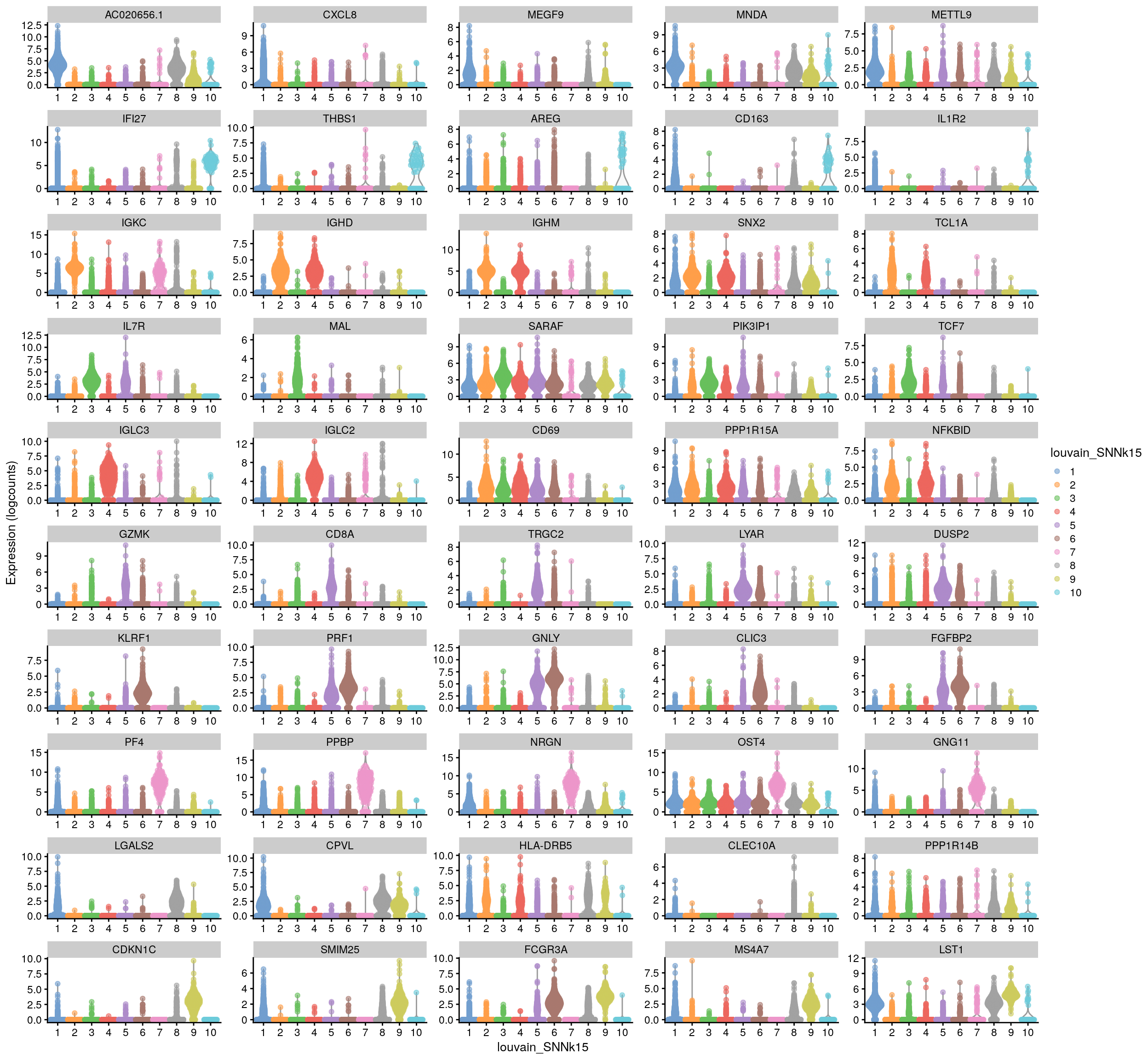
2 DGE across conditions
The second way of computing differential expression is to answer which genes are differentially expressed within a cluster. For example, in our case we have libraries comming from patients and controls and we would like to know which genes are influenced the most in a particular cell type. For this end, we will first subset our data for the desired cell cluster, then change the cell identities to the variable of comparison (which now in our case is the type, e.g. Covid/Ctrl).
# Filter cells from that cluster
cell_selection <- sce[, sce$louvain_SNNk15 == 8]

# Compute differentiall expression
DGE_cell_selection <- findMarkers(
    x = cell_selection,
    groups = cell_selection@colData$type,
    lfc = .25,
    pval.type = "all",
    direction = "any"
)
top5_cell_selection <- lapply(names(DGE_cell_selection), function(x) {
    temp <- DGE_cell_selection[[x]][1:5, 1:2]
    temp$gene <- rownames(DGE_cell_selection[[x]])[1:5]
    temp$cluster <- x
    return(temp)
})
top5_cell_selection <- as_tibble(do.call(rbind, top5_cell_selection))
top5_cell_selection
We can now plot the expression across the type.
scater::plotExpression(cell_selection, features = unique(top5_cell_selection$gene), x = "type", ncol = 5, colour_by = "type")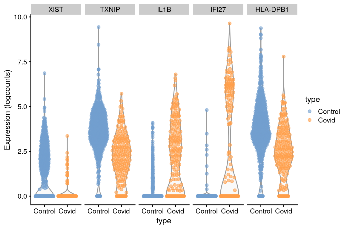
#DGE_ALL6.2:
plotlist <- list()
for (i in unique(top5_cell_selection$gene)) {
    plotlist[[i]] <- plotReducedDim(sce, dimred = "UMAP_on_MNN", colour_by = i, by_exprs_values = "logcounts") +
        ggtitle(label = i) + theme(plot.title = element_text(size = 20))
}
wrap_plots(plotlist, ncol = 3)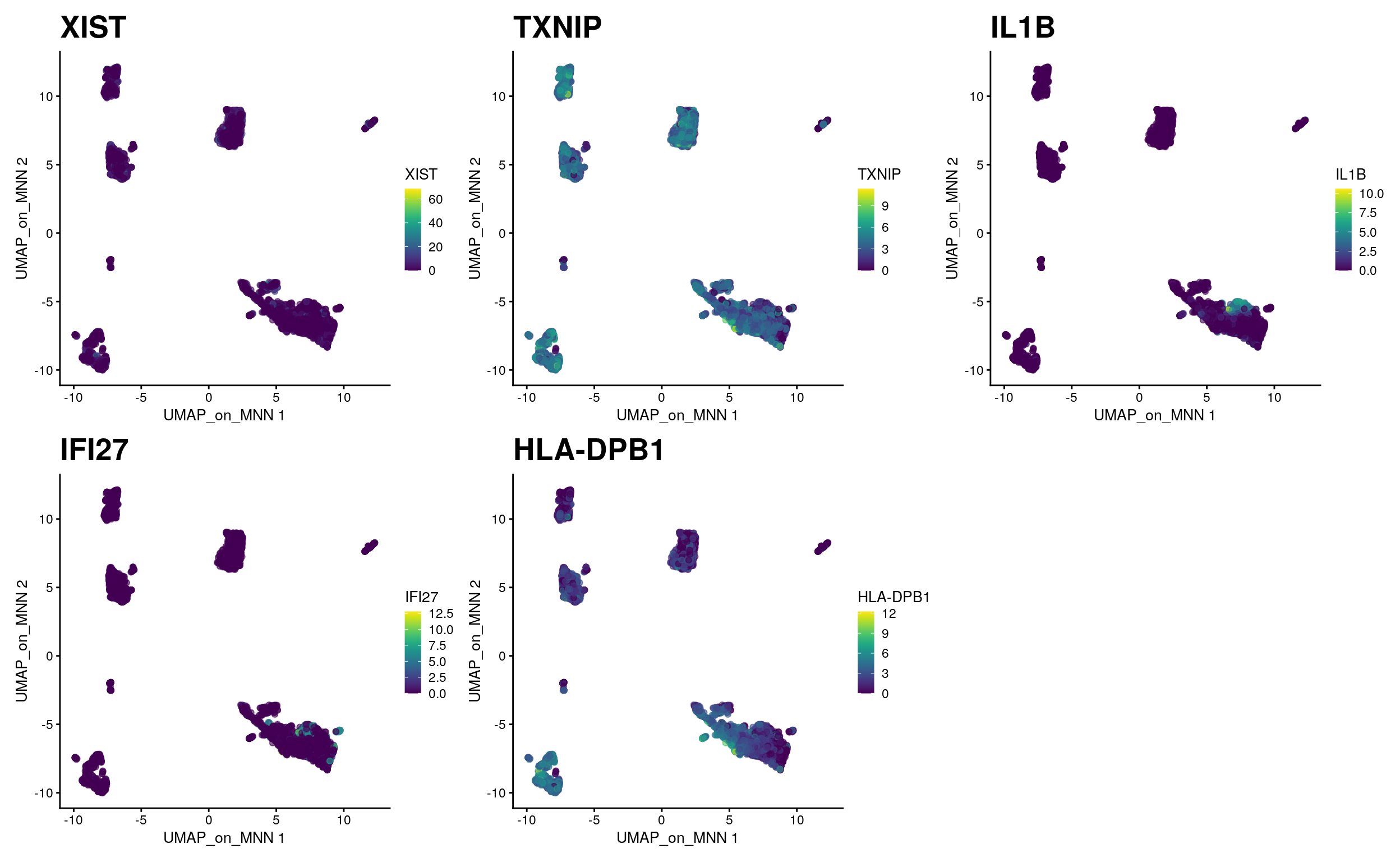
3 Gene Set Analysis (GSA)
3.1 Hypergeometric enrichment test
Having a defined list of differentially expressed genes, you can now look for their combined function using hypergeometric test.
# Load additional packages
library(enrichR)

# Check available databases to perform enrichment (then choose one)
enrichR::listEnrichrDbs()
# Perform enrichment
top_DGE <- DGE_cell_selection$Covid[(DGE_cell_selection$Covid$p.value < 0.01) & (abs(DGE_cell_selection$Covid[, grep("logFC.C", colnames(DGE_cell_selection$Covid))]) > 0.25), ]
enrich_results <- enrichr(
genes = rownames(top_DGE),
databases = "GO_Biological_Process_2017b"
)[[1]]Uploading data to Enrichr... Done.
Querying GO_Biological_Process_2017b... Done.
Parsing results... Done.Some databases of interest:
GO_Biological_Process_2017bKEGG_2019_HumanKEGG_2019_MouseWikiPathways_2019_HumanWikiPathways_2019_Mouse
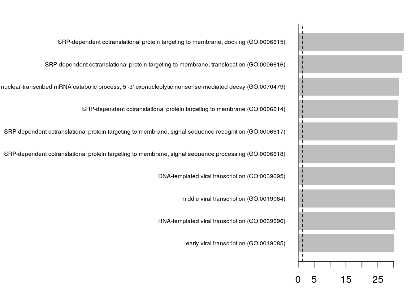
You visualize your results using a simple barplot, for example:
{
    par(mfrow = c(1, 1), mar = c(3, 25, 2, 1))
    barplot(
        height = -log10(enrich_results$P.value)[10:1],
        names.arg = enrich_results$Term[10:1],
        horiz = TRUE,
        las = 1,
        border = FALSE,
        cex.names = .6
    )
    abline(v = c(-log10(0.05)), lty = 2)
    abline(v = 0, lty = 1)
}
4 Gene Set Enrichment Analysis (GSEA)
Besides the enrichment using hypergeometric test, we can also perform gene set enrichment analysis (GSEA), which scores ranked genes list (usually based on fold changes) and computes permutation test to check if a particular gene set is more present in the Up-regulated genes, among the DOWN_regulated genes or not differentially regulated.
# Create a gene rank based on the gene expression fold change
gene_rank <- setNames(DGE_cell_selection$Covid[, grep("logFC.C", colnames(DGE_cell_selection$Covid))], casefold(rownames(DGE_cell_selection$Covid), upper = T))
Once our list of genes are sorted, we can proceed with the enrichment itself. We can use the package to get gene set from the Molecular Signature Database (MSigDB) and select KEGG pathways as an example.
library(msigdbr)

# Download gene sets
msigdbgmt <- msigdbr::msigdbr("Homo sapiens")
msigdbgmt <- as.data.frame(msigdbgmt)

# List available gene sets
unique(msigdbgmt$gs_subcat)
[1] "MIR:MIR_Legacy" "TFT:TFT_Legacy" "CGP" "TFT:GTRD"
[5] "" "VAX" "CP:BIOCARTA" "CGN"
[9] "GO:BP" "GO:CC" "IMMUNESIGDB" "GO:MF"
[13] "HPO" "CP:KEGG" "MIR:MIRDB" "CM"
[17] "CP" "CP:PID" "CP:REACTOME" "CP:WIKIPATHWAYS"# Subset which gene set you want to use.
msigdbgmt_subset <- msigdbgmt[msigdbgmt$gs_subcat == "CP:WIKIPATHWAYS", ]
gmt <- lapply(unique(msigdbgmt_subset$gs_name), function(x) {
msigdbgmt_subset[msigdbgmt_subset$gs_name == x, "gene_symbol"]
})
names(gmt) <- unique(paste0(msigdbgmt_subset$gs_name, "_", msigdbgmt_subset$gs_exact_source))Next, we will run GSEA. This will result in a table containing information for several pathways. We can then sort and filter those pathways to visualize only the top ones. You can select/filter them by either p-value or normalized enrichment score (NES).
library(fgsea)

# Perform enrichemnt analysis
fgseaRes <- fgsea(pathways = gmt, stats = gene_rank, minSize = 15, maxSize = 500, nperm = 10000)
fgseaRes <- fgseaRes[order(fgseaRes$NES, decreasing = T), ]

# Filter the results table to show only the top 10 UP or DOWN regulated processes (optional)
top10_UP <- fgseaRes$pathway[1:10]

# Nice summary table (shown as a plot)
plotGseaTable(gmt[top10_UP], gene_rank, fgseaRes, gseaParam = 0.5)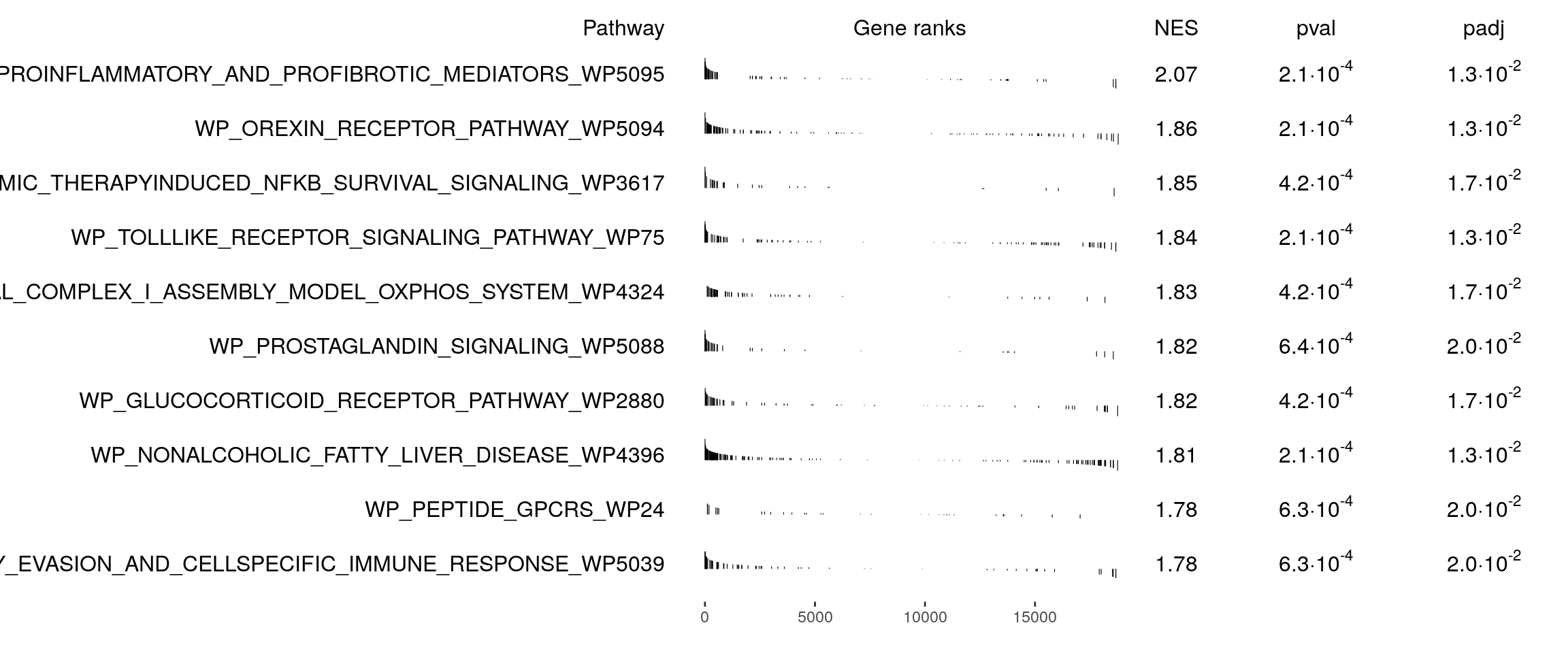
Discuss
Which KEGG pathways are upregulated in this cluster? Which KEGG pathways are dowregulated in this cluster? Change the pathway source to another gene set (e.g. CP:WIKIPATHWAYS or CP:REACTOME or CP:BIOCARTA or GO:BP) and check the if you get similar results?
Finally, let’s save the integrated data for further analysis.
saveRDS(sce, "data/covid/results/bioc_covid_qc_dr_int_cl_dge.rds")5 Session info
Click here
sessionInfo()R version 4.3.0 (2023-04-21)
Platform: x86_64-pc-linux-gnu (64-bit)
Running under: Ubuntu 22.04.3 LTS
Matrix products: default
BLAS: /usr/lib/x86_64-linux-gnu/openblas-pthread/libblas.so.3
LAPACK: /usr/lib/x86_64-linux-gnu/openblas-pthread/libopenblasp-r0.3.20.so; LAPACK version 3.10.0
locale:
[1] LC_CTYPE=en_US.UTF-8 LC_NUMERIC=C
[3] LC_TIME=en_US.UTF-8 LC_COLLATE=en_US.UTF-8
[5] LC_MONETARY=en_US.UTF-8 LC_MESSAGES=en_US.UTF-8
[7] LC_PAPER=en_US.UTF-8 LC_NAME=C
[9] LC_ADDRESS=C LC_TELEPHONE=C
[11] LC_MEASUREMENT=en_US.UTF-8 LC_IDENTIFICATION=C
time zone: Etc/UTC
tzcode source: system (glibc)
attached base packages:
[1] stats4 stats graphics grDevices utils datasets methods
[8] base
other attached packages:
[1] fgsea_1.28.0 msigdbr_7.5.1
[3] enrichR_3.2 dplyr_1.1.2
[5] igraph_1.4.3 pheatmap_1.0.12
[7] patchwork_1.1.2 scran_1.30.0
[9] scater_1.30.1 ggplot2_3.4.2
[11] scuttle_1.12.0 SingleCellExperiment_1.24.0
[13] SummarizedExperiment_1.32.0 Biobase_2.62.0
[15] GenomicRanges_1.54.1 GenomeInfoDb_1.38.5
[17] IRanges_2.36.0 S4Vectors_0.40.2
[19] BiocGenerics_0.48.1 MatrixGenerics_1.14.0
[21] matrixStats_1.0.0
loaded via a namespace (and not attached):
[1] bitops_1.0-7 gridExtra_2.3
[3] rlang_1.1.1 magrittr_2.0.3
[5] compiler_4.3.0 DelayedMatrixStats_1.24.0
[7] vctrs_0.6.2 pkgconfig_2.0.3
[9] crayon_1.5.2 fastmap_1.1.1
[11] XVector_0.42.0 labeling_0.4.2
[13] utf8_1.2.3 rmarkdown_2.22
[15] ggbeeswarm_0.7.2 xfun_0.39
[17] bluster_1.12.0 WriteXLS_6.4.0
[19] zlibbioc_1.48.0 beachmat_2.18.0
[21] jsonlite_1.8.5 DelayedArray_0.28.0
[23] BiocParallel_1.36.0 irlba_2.3.5.1
[25] parallel_4.3.0 cluster_2.1.4
[27] R6_2.5.1 RColorBrewer_1.1-3
[29] limma_3.58.1 Rcpp_1.0.10
[31] knitr_1.43 Matrix_1.5-4
[33] tidyselect_1.2.0 rstudioapi_0.14
[35] abind_1.4-5 yaml_2.3.7
[37] viridis_0.6.3 codetools_0.2-19
[39] curl_5.0.1 lattice_0.21-8
[41] tibble_3.2.1 withr_2.5.0
[43] evaluate_0.21 pillar_1.9.0
[45] generics_0.1.3 RCurl_1.98-1.12
[47] sparseMatrixStats_1.14.0 munsell_0.5.0
[49] scales_1.2.1 glue_1.6.2
[51] metapod_1.10.1 tools_4.3.0
[53] data.table_1.14.8 BiocNeighbors_1.20.2
[55] ScaledMatrix_1.10.0 locfit_1.5-9.8
[57] babelgene_22.9 fastmatch_1.1-3
[59] cowplot_1.1.1 grid_4.3.0
[61] edgeR_4.0.7 colorspace_2.1-0
[63] GenomeInfoDbData_1.2.11 beeswarm_0.4.0
[65] BiocSingular_1.18.0 vipor_0.4.5
[67] cli_3.6.1 rsvd_1.0.5
[69] fansi_1.0.4 S4Arrays_1.2.0
[71] viridisLite_0.4.2 gtable_0.3.3
[73] digest_0.6.31 SparseArray_1.2.3
[75] ggrepel_0.9.3 dqrng_0.3.0
[77] rjson_0.2.21 htmlwidgets_1.6.2
[79] farver_2.1.1 htmltools_0.5.5
[81] lifecycle_1.0.3 httr_1.4.6
[83] statmod_1.5.0