scRNA-seq Integration & Batch correction

Multi-sample/batch harmonization

Aditya Singh

14-Apr-2026

Overview: Why Integration?

The Challenge:

• Comparing cells across individuals/conditions
• Multiple scRNA-seq experiments from different batches
• Technical variations overshadow biological signals
• Need unified analysis across samples

Batch Effects Include:

• Multiple seq runs
• Library preparation protocols
• Platform variations
• Sample handling differences
• And (sadly) many more!

Key challenge: Distinguish biological variation from batch effects

Key Assumption: Batches are uncorrelated (orthogonal) to the variable of interest.

Integration vs Batch Correction

Code

%%{init: {'theme':'base', 'themeVariables': { 'fontSize': '14px', 'primaryTextColor':'#333'}}}%%
flowchart LR
  B["Multiple<br/>Datasets?"]
  
  B --> X["Same<br/>Experiment"]
  X --> C["🔗<br/>INTEGRATION"]
  
  B --> Y["Multiple<br/>Experiments"]
  Y --> D["🧹<br/>BATCH<br/>CORRECTION"]
  Y --> C
  
  C --> C1["Align<br/>Biological<br/>Signals"]
  C1 --> C3["Unified<br/>Cell Types"]
  
  D --> D1["Remove<br/>Technical<br/>Noise"]
  D1 --> D3["Clean<br/>Expression"]
  
  C3 --> E["Proceed to<br/>Analysis"]
  D3 --> E

  classDef decision fill:#e1f5fe,color:#000
  classDef action fill:#f3e5f5,color:#000
  classDef result fill:#e8f5e8,color:#000
  
  class B decision
  class X,Y,D,C action
  class C1,D1,E,C3,D3 result

  linkStyle default stroke:#333,stroke-width:3px

%%{init: {'theme':'base', 'themeVariables': { 'fontSize': '14px', 'primaryTextColor':'#333'}}}%%
flowchart LR
  B["Multiple<br/>Datasets?"]
  
  B --> X["Same<br/>Experiment"]
  X --> C["🔗<br/>INTEGRATION"]
  
  B --> Y["Multiple<br/>Experiments"]
  Y --> D["🧹<br/>BATCH<br/>CORRECTION"]
  Y --> C
  
  C --> C1["Align<br/>Biological<br/>Signals"]
  C1 --> C3["Unified<br/>Cell Types"]
  
  D --> D1["Remove<br/>Technical<br/>Noise"]
  D1 --> D3["Clean<br/>Expression"]
  
  C3 --> E["Proceed to<br/>Analysis"]
  D3 --> E

  classDef decision fill:#e1f5fe,color:#000
  classDef action fill:#f3e5f5,color:#000
  classDef result fill:#e8f5e8,color:#000
  
  class B decision
  class X,Y,D,C action
  class C1,D1,E,C3,D3 result

  linkStyle default stroke:#333,stroke-width:3px

• Batch correction is a type of integration; vice versa is not true
• In practice, integration = batch correction + dataset merging
• If batch correction is needed, it’s done along with the integration of samples
  • Multiple samples integration is almost always performed
  • Batch correction is added to it only when needed

Closer look

Image adapted from Argelaguet et al. (2021).

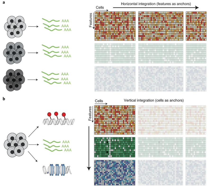
• Panel “a”: Same type of data (scRNAseq)
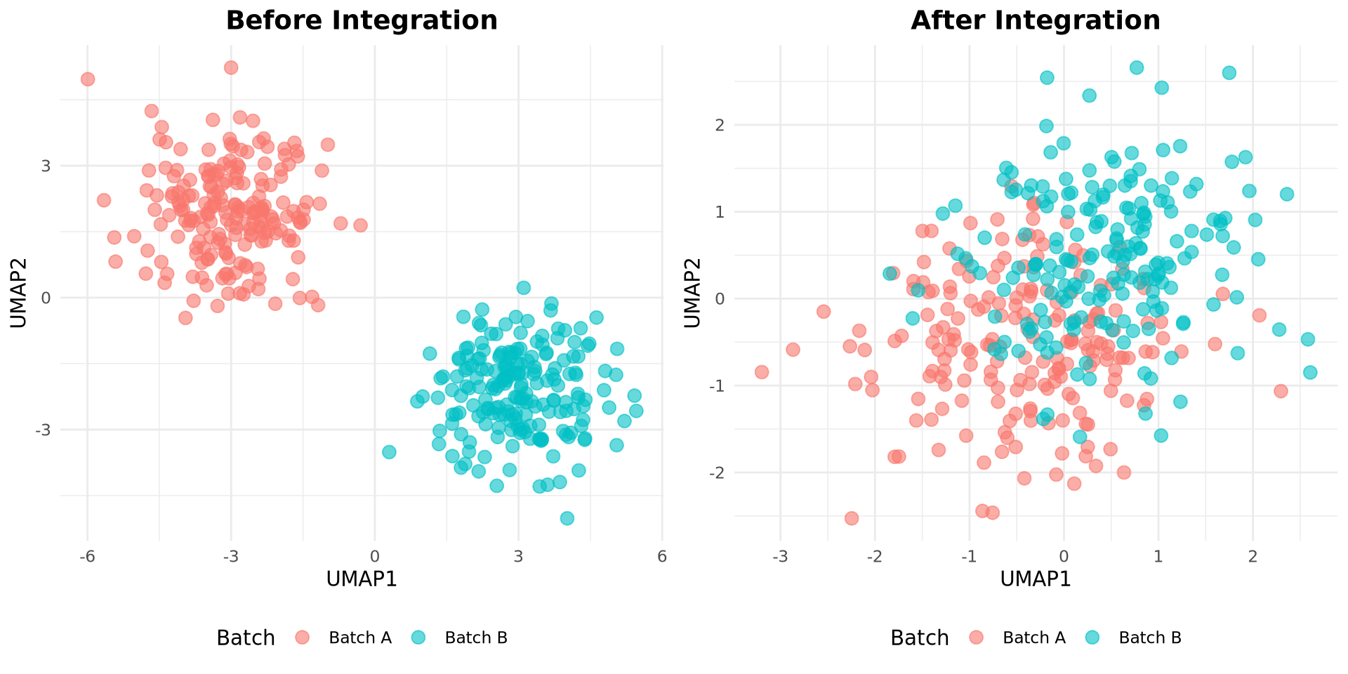
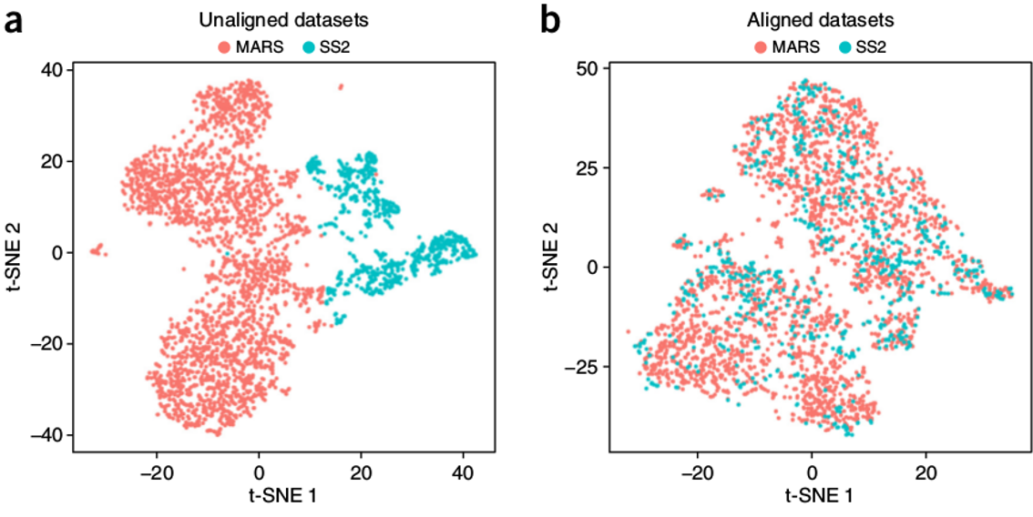
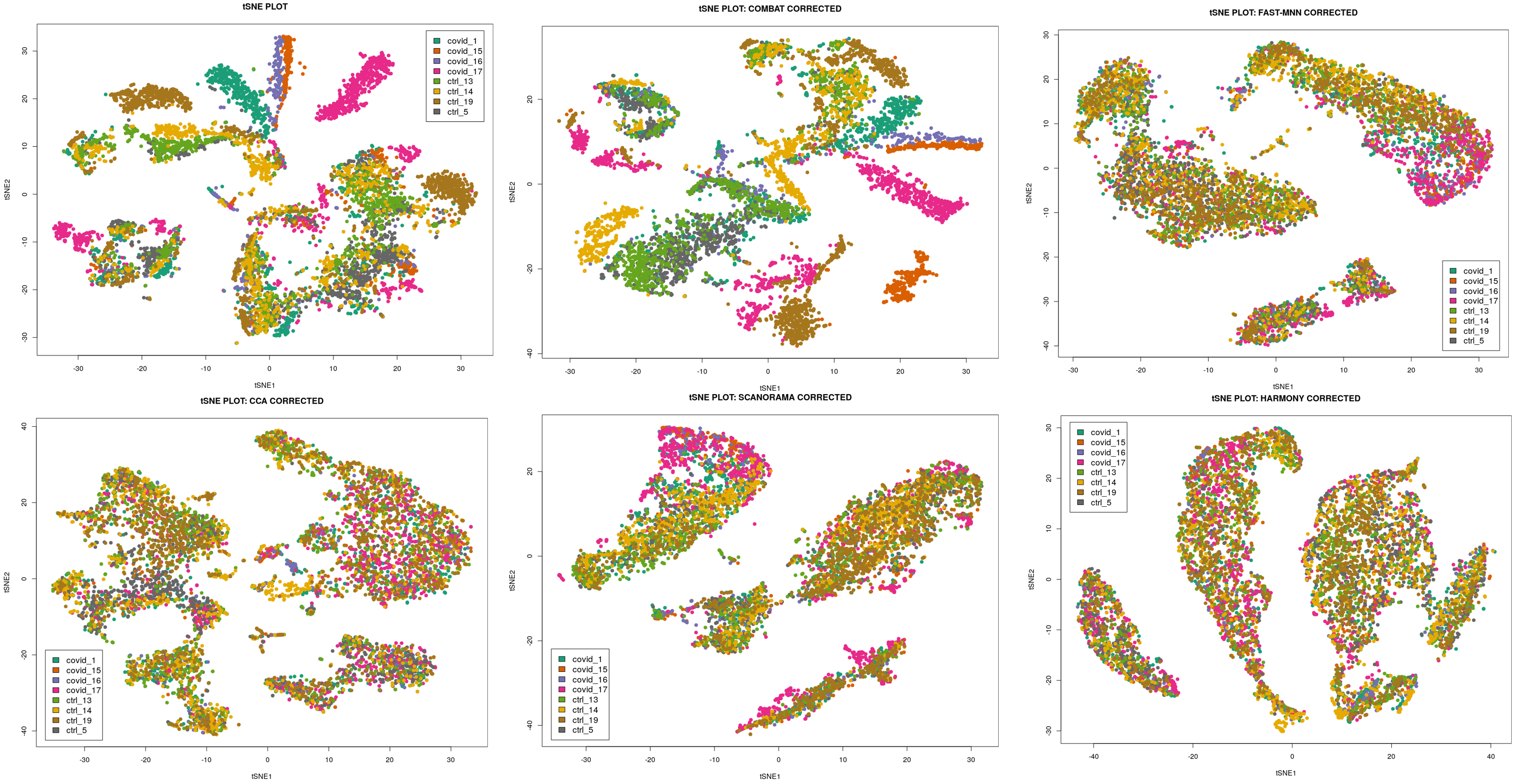
  • Integration & batch-correction (BC)
  • 3 samples same run: Without BC
  • 3 samples 2 batches: With BC
• Panel “b”: Multi-omics Integration
  • Same samples, multiple platforms
  • Example: RNAseq + ATACseq
  • Beyond scope here
  • Good to know and not to confuse

Orthogonal Assumption

✅ Better Design

Balanced Batches

Sample	Condition	Batch
Patient A	Control	1
Patient B	Control	2
Patient C	Control	3
Patient D	Treated	1
Patient E	Treated	2
Patient F	Treated	3

❌ Bad Design

Confounded Batches

Sample	Condition	Batch
Patient A	Control	1
Patient B	Control	1
Patient C	Control	1
Patient D	Treated	2
Patient E	Treated	2
Patient F	Treated	2

Overview of Integration Methods

Method	Algorithm	Language	Library	Ref
CCA	Canonical Correlation Analysis	R	Seurat	Cell 2019
MNN	Mutual Nearest Neighbors correction	R / Python	scater / Scanpy	Nat. Biotech 2018
Conos	Graph-based joint kNN alignment	R	conos	Nat. Methods 2019
Harmony	Iterative PC correction (soft-clustering)	R / Python	harmony/ harmonypy	Nat. Methods 2019
Scanorama	Manifold alignment + SVD-based merging	Python	scanorama	Nat. Biotech 2019

Note: This is not an exhaustive list, just a selection of popular methods that we’ll cover in the exercises

Classic Batch Correction Methods

Method	Algorithm	Language	Library	Ref
ComBat	Empirical Bayes location/scale adjustment	R	sva	Bioinformatics 2007
ComBat-seq	Negative binomial ComBat for counts	R	ComBat_seq	NAR Genomics 2020
limma	Linear models with empirical Bayes	R	limma	NAR 2015
RUVSeq	Remove unwanted variation (factor-based)	R	RUVSeq	BMC Bioinf 2016
SVA	Surrogate variable analysis	R	sva	PNAS 2017
ZINB-WaVE	Zero-inflated negative binomial	R	zinbwave	Genome Biol 2017

Note: These methods were developed for bulk data and usually not perform well on scRNA-seq due to sparsity and zero-inflation. They are included here for context

AI/Deep Learning Integration Methods

Method	Algorithm	Language	Library	Ref
scVI	Variational autoencoder	Python	scvi-tools	Nat Biotech 2022
scANVI	Conditional variational autoencoder	Python	scvi-tools	Nat Methods 2021
scGen	Causal VAE for perturbation modeling	Python	scgen	Nat Methods 2019
SAUCIE	Self-supervised autoencoder	Python	SAUCIE	Nat Methods 2019
DESC	Deep embedded single cell clustering	Python	DESC	Nat Communs 2020

Note: These methods are powerful but often require more computational resources and expertise to use effectively. Watch this space, future might be here!

CCA: Canonical Correlation Analysis

CCA: finding shared correlated components across batches.

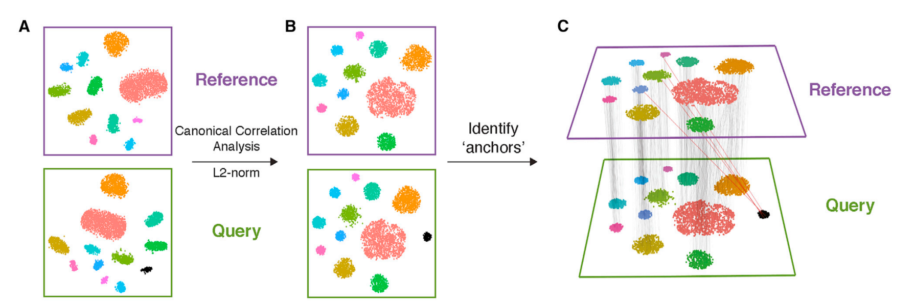
• Finds correlated features between batches
• Creates canonical variates capturing shared variation
• Projects cells into aligned latent space
• Linear approach - computationally efficient for large datasets

Mutual Nearest Neighbors (MNN) Integration

• Core concept: Identifies pairs of cells that are each other’s nearest neighbors across batches in high-dimensional gene expression space

  • Assumes shared cell types exist between batches
  • Doesn’t require identical population composition

• No predefined populations needed: Works without cell type annotations

• How it works:

  • Computes kNN graphs in PCA space
  • Finds mutual nearest neighbor pairs across batches
  • Applies linear batch-effect corrections using correction vectors

• Minimal biological artifacts: Conservative approach, reducing risk of removing biological differences

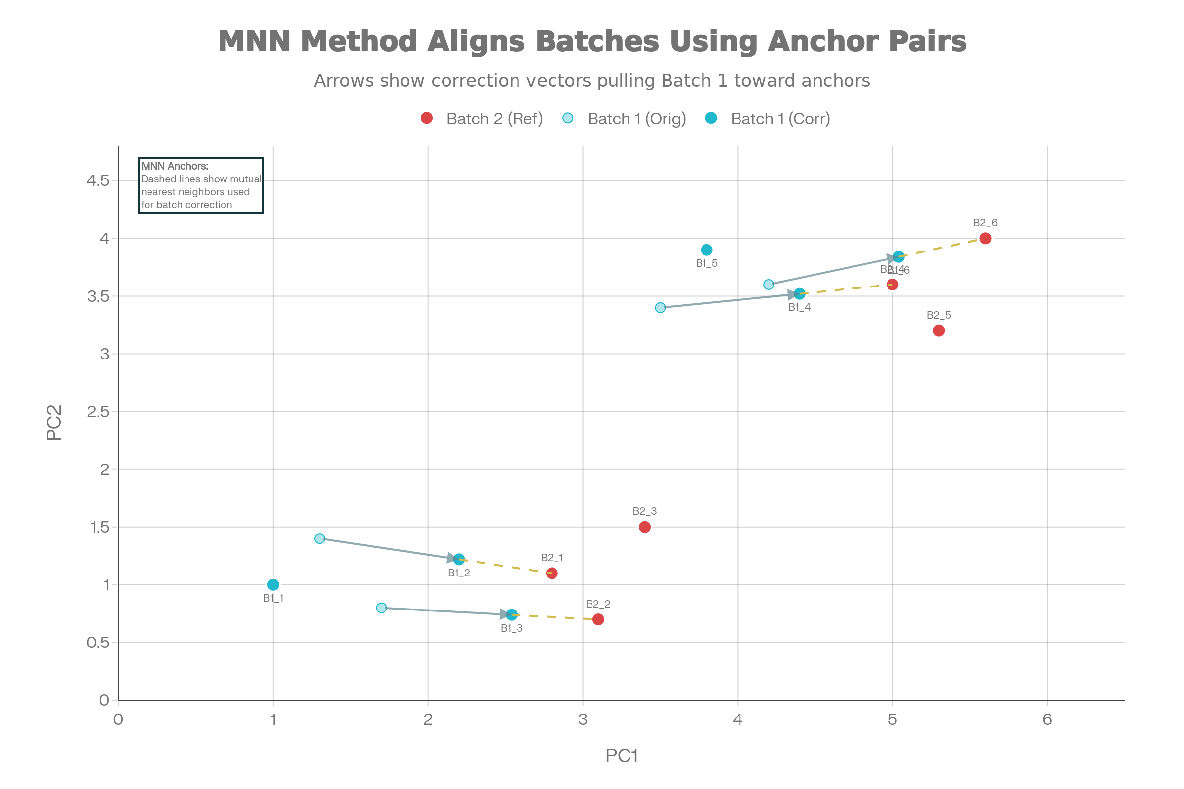
Visualizing MNN Correction

MNN integration example

Harmony: Iterative PC Correction

Image from Korsunsky et al. (2019).

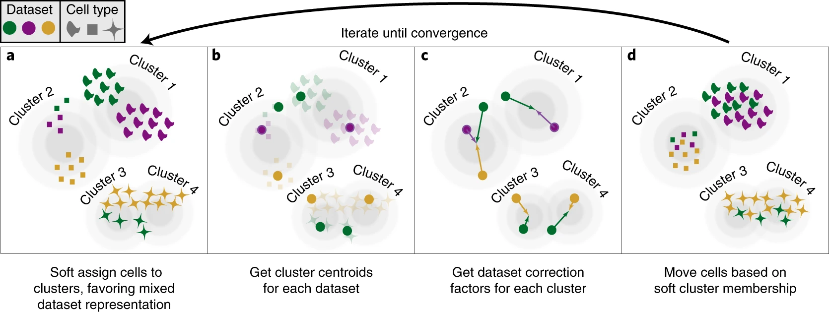
Harmony iteratively adjusts cell embeddings so that each cluster contains a balanced mix of batches

Scanorama: Manifold Alignment + SVD

Image from Hie et al. (2019).

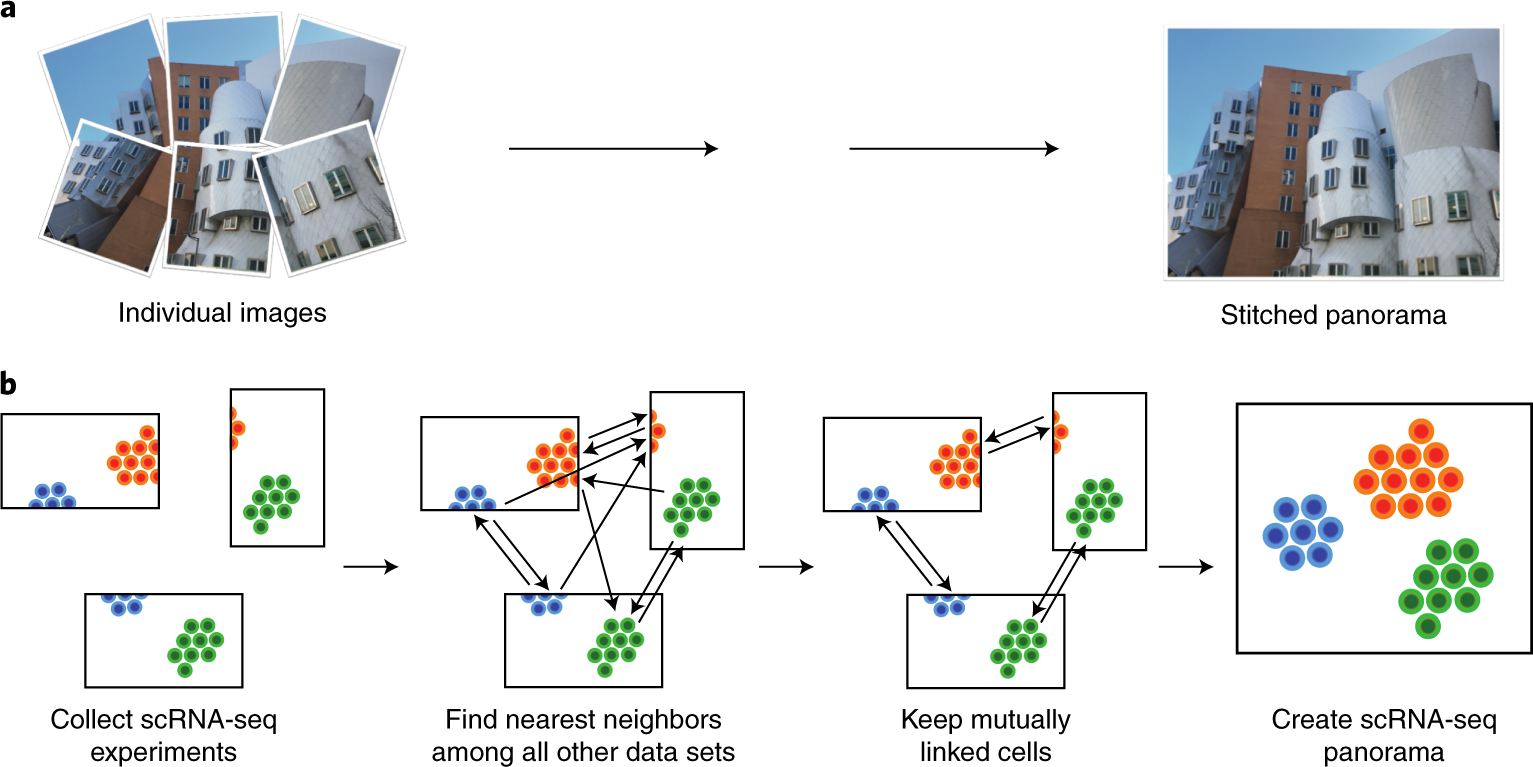
• Builds manifold alignment between pairs of datasets
• Uses Singular Value Decomposition (SVD) for efficient merging
• Iteratively corrects and merges multiple datasets

Conos: Graph-Based Alignment

Conos Barkas et al. (2019).

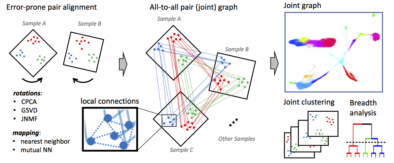
• Builds separate k-NN graphs for each sample
• Constructs joint graph by adding cross-sample edges between similar cells
• Preserves per-sample structure while enabling global analysis
• Particularly useful for many-sample studies with distinct biological states

Comparison

Credit: Nikolay Oskolov

Comparison Matrix

Aspect	CCA	MNN	Harmony	Scanorama	Conos
Speed	Fast	Slow	Fast	Medium	Slow
Scalability	~10k	~50k	125k+	~50k	~30k
Batch Correction	Good	Excellent	Good	Excellent	Very Good
Biology Preservation	Medium	Excellent	Excellent	Good	Excellent
Rare Type Detection	Poor	Excellent	Good	Medium	Good
Learning Curve	Low	Medium	Low	Medium	High
Language	R	R/Python	R/Python	Python	R
Graph-Based	No	No	No	No	Yes

Benchmark References for Comparison Table

Claim	Source	Key Finding
Speed: Harmony > CCA > Scanorama > MNN > Conos	Tran et al. (2020)	Harmony 30-200x faster than MNN at 500k cells
Scalability: Harmony(125k+) > MNN/Scanorama(50k) > CCA(10k)	Korsunsky et al. (2019)	Harmony scales to 1M+ cells, MNN fails >50k
Batch Correction: MNN/Scanorama > Conos > Harmony > CCA	Luecken et al. (2022)	MNN/Scanorama top kBET/LISI scores
Biology Preservation: MNN/Harmony/Conos > Scanorama > CCA	Luecken et al. (2022)	MNN best cell-cycle/trajectory conservation
Rare Type Detection: MNN superior	Distilled information	MNN being local correction, preserves rare populations
Learning Curve: CCA/Harmony < MNN/Scanorama < Conos	Personal opinion	Harmony/CCA: simple params; Conos: complex graphs

Best Practices

• Feature selection: Use highly variable genes (2000-3000) before integration
• Batch awareness: Always specify batch variable during integration
• QC first: Remove low-quality cells before integration
• Metrics matter: Assess both batch mixing and biological preservation
• Visualize results: Check UMAP, violin plots by batch, cell type distribution
• Validate: Confirm known biology is preserved in integrated data
• Don’t fix something unbroken: Make sure there are batch effects before “fixing”

Common Pitfalls

Overcorrection

• Removing real biological signal
• Check with known marker genes

Batch structure ignored

• Not specifying batch variable correctly
• Can lead to suboptimal integration

Incompatible preprocessing

• Different normalization or scaling across batches
• Standardize preprocessing pipeline first

Confounded design

• Batch perfectly correlated with condition (eg. all controls in batch 1, all treated in batch 2)
• Integration cannot disentangle technical vs biological variation

Q&A

Key takeaway: Integration balances batch removal with biology preservation

Summary slides for revision follow

Summary: Integration goals

Q1. What is the main goal of scRNA-seq integration?

A: To align cells so they group by biological signal (for example, cell type) rather than technical or sample-specific differences.

Q2. Why can integration be needed even with one sequencing batch?

A: Different samples in the same run can still differ in preparation, dissociation, or depth, making cells cluster by sample instead of cell type.

Q3. What pattern in a UMAP suggests batch effect problems?

A: Clusters separate mainly by batch label even though the same cell type exists in all batches.

Summary: CCA / Seurat anchors

Q4. Conceptually, what does CCA do for integration?

A: It finds shared low-dimensional “correlated directions” across datasets where similar cell states align.

Q5. What are “anchors” in Seurat’s CCA-based integration?

A: Pairs or small groups of cells from different datasets that represent the same biological state and are used as reference points for alignment.

Q6. Simple example

A: Take T cells from patient A and B that look similar, treat them as anchors, and warp both datasets so T cells from A and B overlap in the joint space.

Summary: Harmony

Q7. What is the core idea behind Harmony?

A: Start in PCA space, then iteratively shift cell embeddings so each cluster has similar contributions from each batch, reducing batch-driven structure.

Q8. Why is Harmony often practical for large datasets?

A: It operates on PCs, is relatively fast, and fits into a simple PCA → Harmony → UMAP workflow.

Q9. Metaphor for Harmony’s adjustment

A: You have groups of similar cells on a map; Harmony gently nudges cells from overrepresented batches so each group has a fair mix of batches.

Summary: MNN & Scanorama

Q10. What is a mutual nearest neighbors (MNN) pair?

A: A pair of cells, one from each dataset, where each is among the nearest neighbors of the other in expression space.

Q11. How does MNN-based integration use these pairs?

A: It assumes MNN pairs represent the same cell state and computes local correction vectors to align the datasets around those pairs.

Q12. Intuitive example for MNN in lecture

A: If a T cell in dataset A and a T cell in dataset B are each other’s closest match, link them and use that link to locally shift one dataset towards the other.

Q13. What is the main idea behind Scanorama?

A: It uses MNN-like matches across many datasets and stitches them together like a panorama to build a unified embedding.

Q14. Why is Scanorama useful for many-dataset studies?

A: It can integrate multiple experiments at once by finding shared cell populations and merging them into a common space.

Summary: Conos

Q15. What is Conos’ high-level approach to integration?

A: It builds a graph for each sample, then constructs a joint graph across samples using cross-sample neighbors, and analyzes this global graph for clustering and alignment.

Q16. When is Conos particularly attractive?

A: When you have many samples and want to keep per-sample identity while still obtaining joint clustering from the combined graph.

Q17. Simple metaphor for Conos

A: Each sample is its own social network; Conos adds edges between similar people across networks and then analyzes the big merged social graph.

Summary: Over- vs under-integration & choice

Q18. How can you spot “over-integration” ?

A: Marker genes lose specificity across clusters, known biology is obscured, and distinct cell types merge together.

Q19. How can you spot “under-integration”?

A: UMAP: If technically distinct groups are not-integrated (eg. sequencing run 1 and 2)

Q20. Simple rule-of-thumb when choosing an integration method

A: Use anchor/CCA or Harmony for typical multi-sample datasets; consider MNN/Scanorama for more local alignment or many datasets; use Conos for graph-based integration across many samples while preserving sample identity.

Resources & Further reading

• Luecken, M.D., Büttner, M., Chaichoompu, K. et al. Benchmarking atlas-level data integration in single-cell genomics. Nat Methods 19, 41–50 (2022). https://doi.org/10.1038/s41592-021-01336-8
• Korsunsky, I., Millard, N., Fan, J. et al. Fast, sensitive and accurate integration of single-cell data with Harmony. Nat Methods 16, 1289–1296 (2019). https://doi.org/10.1038/s41592-019-0619-0
• Hie, B., Bryson, B. & Berger, B. Efficient integration of heterogeneous single-cell transcriptomes using Scanorama. Nat Biotechnol 37, 685–691 (2019). https://doi.org/10.1038/s41587-019-0113-3
• Argelaguet, R., Velten, B., Arnol,D, S. et al. Multi-omics factor analysis—a framework for unsupervised integration of multi-omics data sets. Mol Syst Biol 14, e8124 (2018). https://doi.org/10.15252/msb.20178124
• Barkas N., Petukhov V., Nikolaeva D., Lozinsky Y., Demharter S., Khodosevich K., & Kharchenko P.V. Joint analysis of heterogeneous single-cell RNA-seq dataset collections. Nature Methods, (2019). https://doi.org/10.1038/s41592-019-0466-z