import numpy as np
import pandas as pd
import scanpy as sc
import gseapy
import matplotlib.pyplot as plt
import warnings
import os
import subprocess

warnings.simplefilter(action="ignore", category=Warning)

# verbosity: errors (0), warnings (1), info (2), hints (3)
sc.settings.verbosity = 2

sc.settings.set_figure_params(dpi=80)
Note
Code chunks run Python commands unless it starts with %%bash, in which case, those chunks run shell commands.
In this tutorial we will cover differential gene expression, which comprises an extensive range of topics and methods. In single cell, differential expresison can have multiple functionalities such as identifying marker genes for cell populations, as well as identifying differentially regulated genes across conditions (healthy vs control). We will also cover controlling batch effect in your test.
Differential expression is performed with the function rank_genes_group. The default method to compute differential expression is the t-test_overestim_var. Other implemented methods are: logreg, t-test and wilcoxon.
By default, the .raw attribute of AnnData is used in case it has been initialized, it can be changed by setting use_raw=False.
The clustering with resolution 0.6 seems to give a reasonable number of clusters, so we will use that clustering for all DE tests.
First, let’s import libraries and fetch the clustered data from the previous lab.
Read in the clustered data object.
# download pre-computed data if missing or long compute
fetch_data = True

# url for source and intermediate data
path_data = "https://nextcloud.dc.scilifelab.se/public.php/webdav"
curl_upass = "zbC5fr2LbEZ9rSE:scRNAseq2025"

path_results = "data/covid/results"
if not os.path.exists(path_results):
    os.makedirs(path_results, exist_ok=True)

# path_file = "data/covid/results/scanpy_covid_qc_dr_int_cl.h5ad"
path_file = "data/covid/results/scanpy_covid_qc_dr_int_cl.h5ad"
if fetch_data and not os.path.exists(path_file):
    file_url = os.path.join(path_data, "covid/results_scanpy/scanpy_covid_qc_dr_int_cl.h5ad")
    subprocess.call(["curl", "-u", curl_upass, "-o", path_file, file_url ])

adata = sc.read_h5ad(path_file)
adata
AnnData object with n_obs × n_vars = 7332 × 19468
obs: 'type', 'sample', 'batch', 'n_genes_by_counts', 'total_counts', 'total_counts_mt', 'pct_counts_mt', 'total_counts_ribo', 'pct_counts_ribo', 'total_counts_hb', 'pct_counts_hb', 'percent_mt2', 'n_counts', 'n_genes', 'percent_chrY', 'XIST-counts', 'S_score', 'G2M_score', 'phase', 'doublet_scores', 'predicted_doublets', 'doublet_info', 'leiden', 'leiden_0.4', 'leiden_0.6', 'leiden_1.0', 'leiden_1.4', 'kmeans5', 'kmeans10', 'kmeans15', 'hclust_5', 'hclust_10', 'hclust_15'
var: 'gene_ids', 'feature_types', 'genome', 'mt', 'ribo', 'hb', 'n_cells_by_counts', 'mean_counts', 'pct_dropout_by_counts', 'total_counts', 'n_cells', 'highly_variable', 'means', 'dispersions', 'dispersions_norm', 'highly_variable_nbatches', 'highly_variable_intersection'
uns: 'dendrogram_leiden_0.6', 'doublet_info_colors', 'hclust_10_colors', 'hclust_15_colors', 'hclust_5_colors', 'hvg', 'kmeans10_colors', 'kmeans15_colors', 'kmeans5_colors', 'leiden', 'leiden_0.4', 'leiden_0.4_colors', 'leiden_0.6', 'leiden_0.6_colors', 'leiden_1.0', 'leiden_1.0_colors', 'leiden_1.4', 'leiden_1.4_colors', 'log1p', 'neighbors', 'pca', 'phase_colors', 'sample_colors', 'tsne', 'umap'
obsm: 'Scanorama', 'X_pca', 'X_pca_harmony', 'X_tsne', 'X_tsne_bbknn', 'X_tsne_harmony', 'X_tsne_scanorama', 'X_tsne_uncorr', 'X_umap', 'X_umap_bbknn', 'X_umap_harmony', 'X_umap_scanorama', 'X_umap_uncorr'
obsp: 'connectivities', 'distances'Check what you have in the different matrices.
print(adata.X.shape)
print(type(adata.raw))
print(adata.X[:10,:10])
(7332, 19468)
<class 'NoneType'>
<Compressed Sparse Row sparse matrix of dtype 'float64'
with 2 stored elements and shape (10, 10)>
Coords Values
(1, 4) 1.479703103222477
(8, 7) 1.6397408237842532As you can see, the X matrix contains all genes and the data looks logtransformed.
For DGE analysis we would like to run with all genes, on normalized values, so if you did subset the adata.X for variable genes you would have to revert back to the raw matrix with adata = adata.raw.to_adata(). In case you have raw counts in the matrix you also have to renormalize and logtransform.
Now lets look at the clustering of the object we loaded in the umap. We will use leiden_0.6 clustering in this exercise. If you recall from the previous exercise, we set the default umap to the umap created with Harmony.
sc.pl.umap(adata, color='leiden_0.6')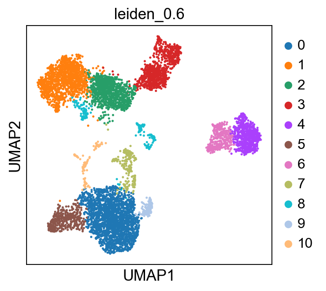
1 T-test
sc.tl.rank_genes_groups(adata, 'leiden_0.6', method='t-test', key_added = "t-test")
sc.pl.rank_genes_groups(adata, n_genes=25, sharey=False, key = "t-test")

# results are stored in the adata.uns["t-test"] slot
adata.uns.keys()
ranking genes
finished (0:00:03)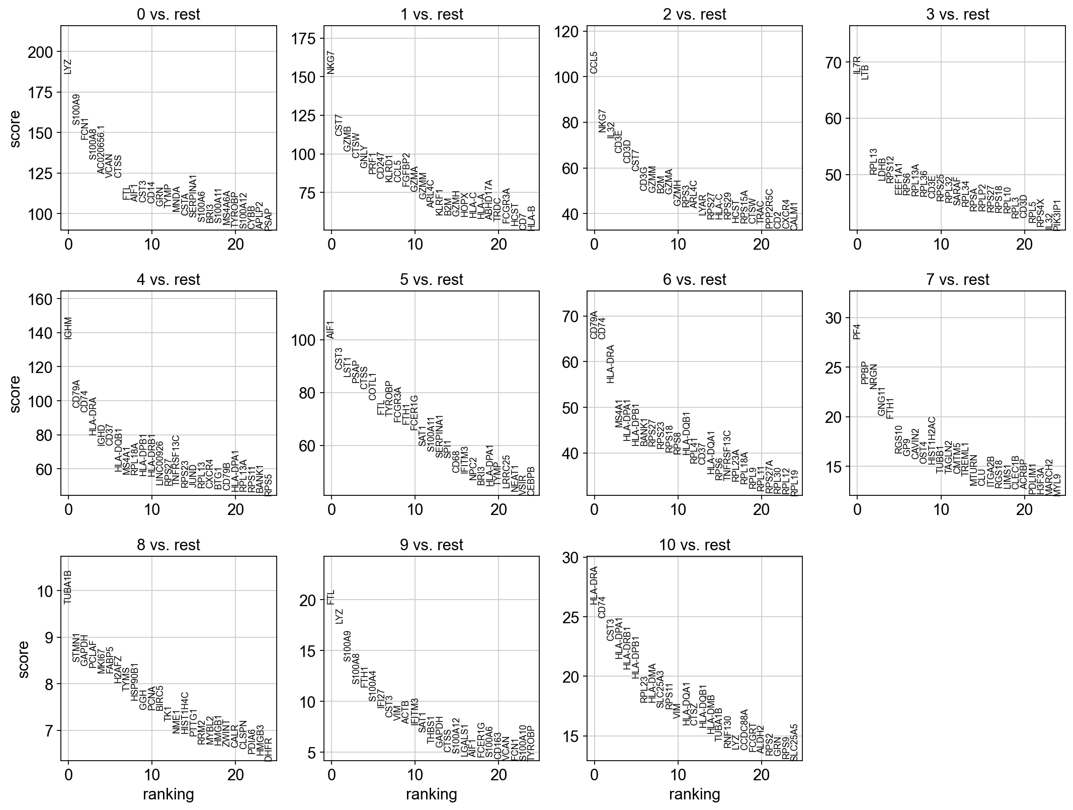
dict_keys(['dendrogram_leiden_0.6', 'doublet_info_colors', 'hclust_10_colors', 'hclust_15_colors', 'hclust_5_colors', 'hvg', 'kmeans10_colors', 'kmeans15_colors', 'kmeans5_colors', 'leiden', 'leiden_0.4', 'leiden_0.4_colors', 'leiden_0.6', 'leiden_0.6_colors', 'leiden_1.0', 'leiden_1.0_colors', 'leiden_1.4', 'leiden_1.4_colors', 'log1p', 'neighbors', 'pca', 'phase_colors', 'sample_colors', 'tsne', 'umap', 't-test'])2 T-test overestimated_variance
sc.tl.rank_genes_groups(adata, 'leiden_0.6', method='t-test_overestim_var', key_added = "t-test_ov")
sc.pl.rank_genes_groups(adata, n_genes=25, sharey=False, key = "t-test_ov")
ranking genes
finished (0:00:00)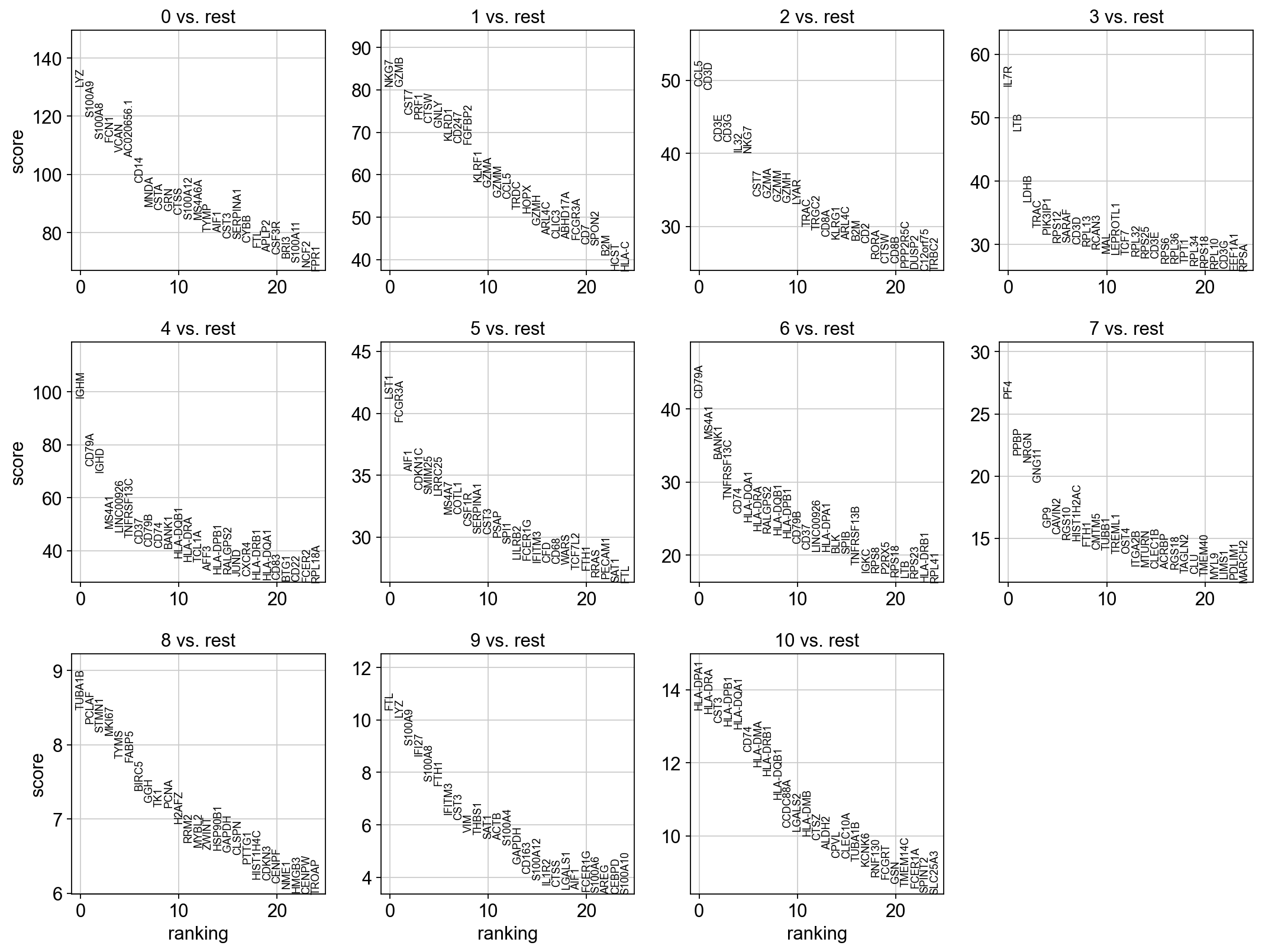
3 Wilcoxon rank-sum
The result of a Wilcoxon rank-sum (Mann-Whitney-U) test is very similar. We recommend using the latter in publications, see e.g., Sonison & Robinson (2018). You might also consider much more powerful differential testing packages like MAST, limma, DESeq2 and, for python, the recent diffxpy.
sc.tl.rank_genes_groups(adata, 'leiden_0.6', method='wilcoxon', key_added = "wilcoxon")
sc.pl.rank_genes_groups(adata, n_genes=25, sharey=False, key="wilcoxon")
ranking genes
finished (0:00:11)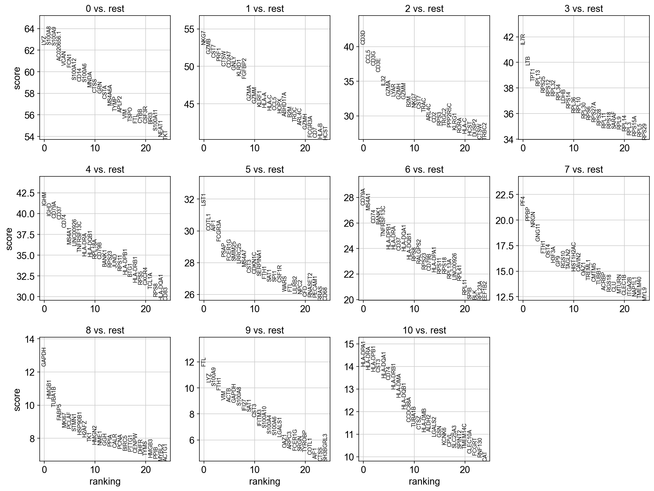
4 Logistic regression test
As an alternative, let us rank genes using logistic regression. For instance, this has been suggested by Natranos et al. (2018). The essential difference is that here, we use a multi-variate appraoch whereas conventional differential tests are uni-variate. Clark et al. (2014) has more details.
sc.tl.rank_genes_groups(adata, 'leiden_0.6', method='logreg',key_added = "logreg")
sc.pl.rank_genes_groups(adata, n_genes=25, sharey=False, key = "logreg")
ranking genes
finished (0:00:20)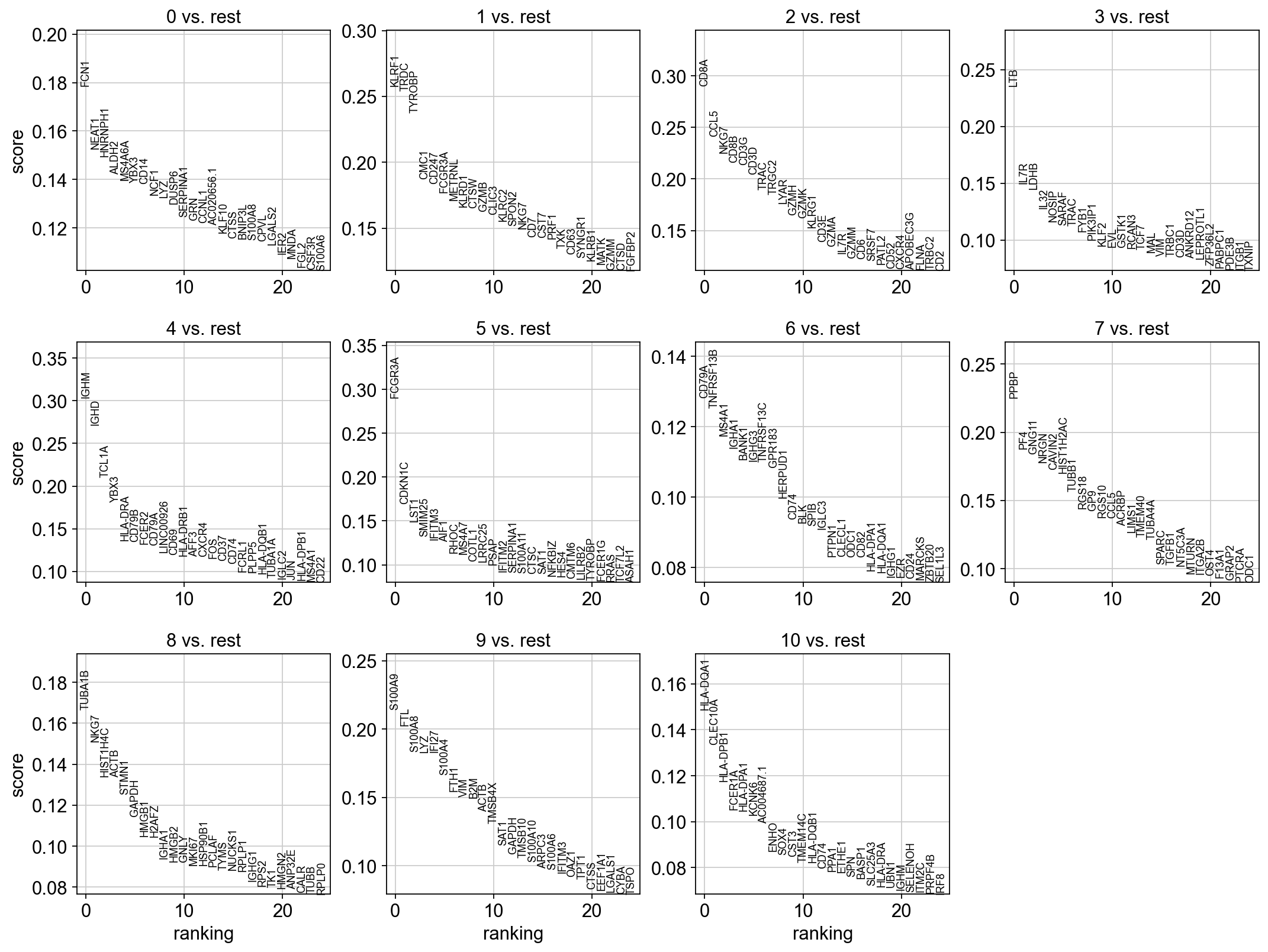
5 Compare genes
Take all significant DE genes for cluster0 with each test and compare the overlap.
#compare cluster1 genes, only stores top 100 by default

wc = sc.get.rank_genes_groups_df(adata, group='0', key='wilcoxon', pval_cutoff=0.01, log2fc_min=0)['names']
tt = sc.get.rank_genes_groups_df(adata, group='0', key='t-test', pval_cutoff=0.01, log2fc_min=0)['names']
tt_ov = sc.get.rank_genes_groups_df(adata, group='0', key='t-test_ov', pval_cutoff=0.01, log2fc_min=0)['names']

from matplotlib_venn import venn3

venn3([set(wc),set(tt),set(tt_ov)], ('Wilcox','T-test','T-test_ov') )
plt.show()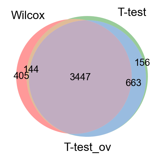
As you can see, the Wilcoxon test and the T-test with overestimated variance gives very similar result. Also the regular T-test has good overlap.
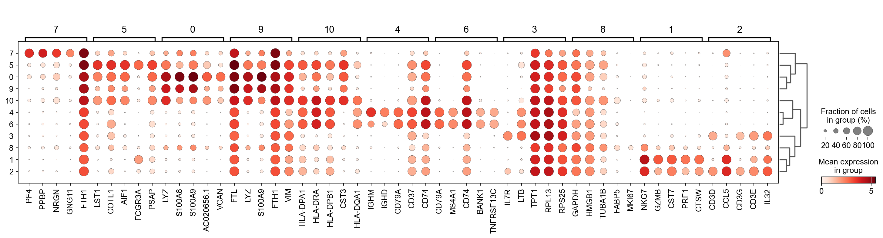
6 Visualization
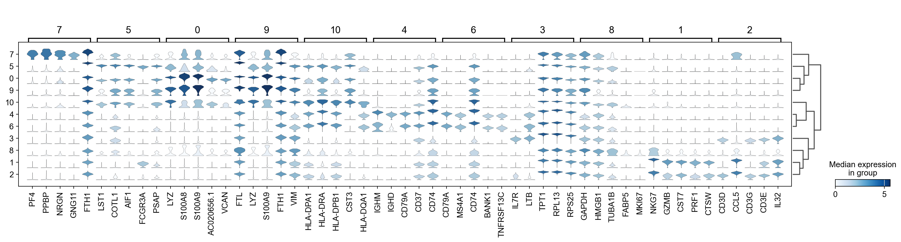
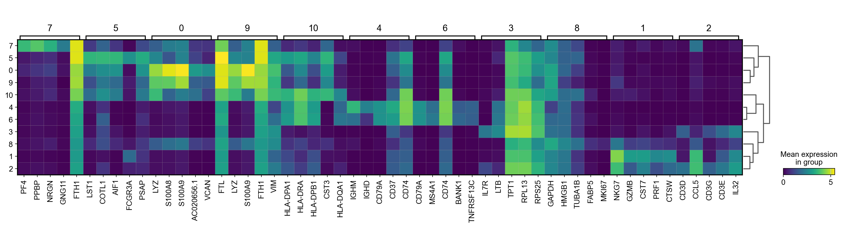
There are several ways to visualize the expression of top DE genes. Here we will plot top 5 genes per cluster from Wilcoxon test as heatmap, dotplot, violin plots or a matrix with average expression.
sc.pl.rank_genes_groups_heatmap(adata, n_genes=5, key="wilcoxon", groupby="leiden_0.6", show_gene_labels=True)
sc.pl.rank_genes_groups_dotplot(adata, n_genes=5, key="wilcoxon", groupby="leiden_0.6")
sc.pl.rank_genes_groups_stacked_violin(adata, n_genes=5, key="wilcoxon", groupby="leiden_0.6")
sc.pl.rank_genes_groups_matrixplot(adata, n_genes=5, key="wilcoxon", groupby="leiden_0.6")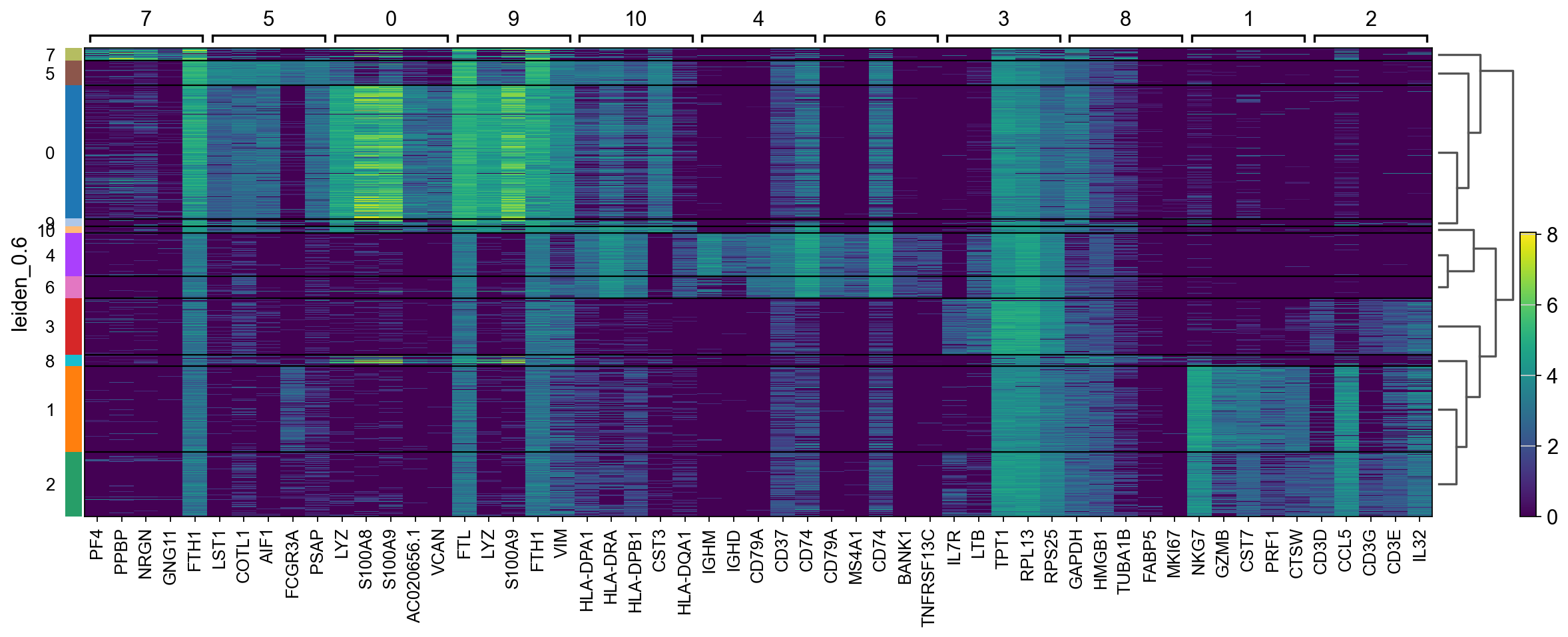
7 Compare specific clusters
We can also do pairwise comparisons of individual clusters on one vs many clusters. For instance, clusters 1 & 2 have very similar expression profiles.
sc.tl.rank_genes_groups(adata, 'leiden_0.6', groups=['1'], reference='2', method='wilcoxon')
sc.pl.rank_genes_groups(adata, groups=['1'], n_genes=20)
ranking genes
finished (0:00:03)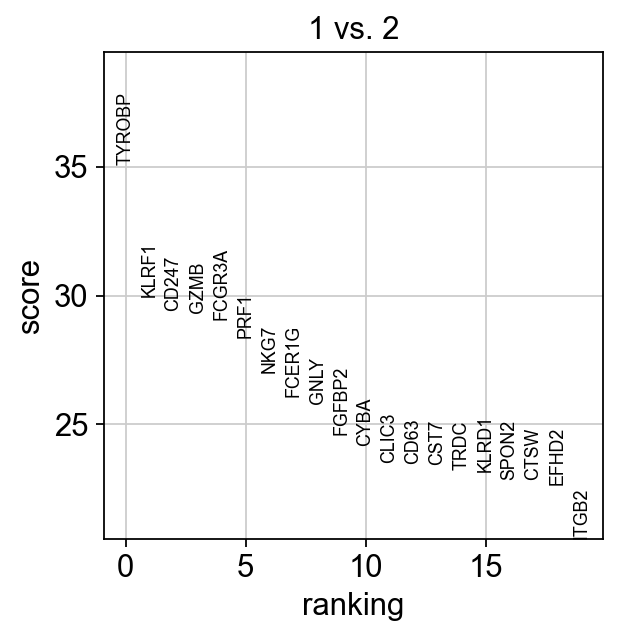
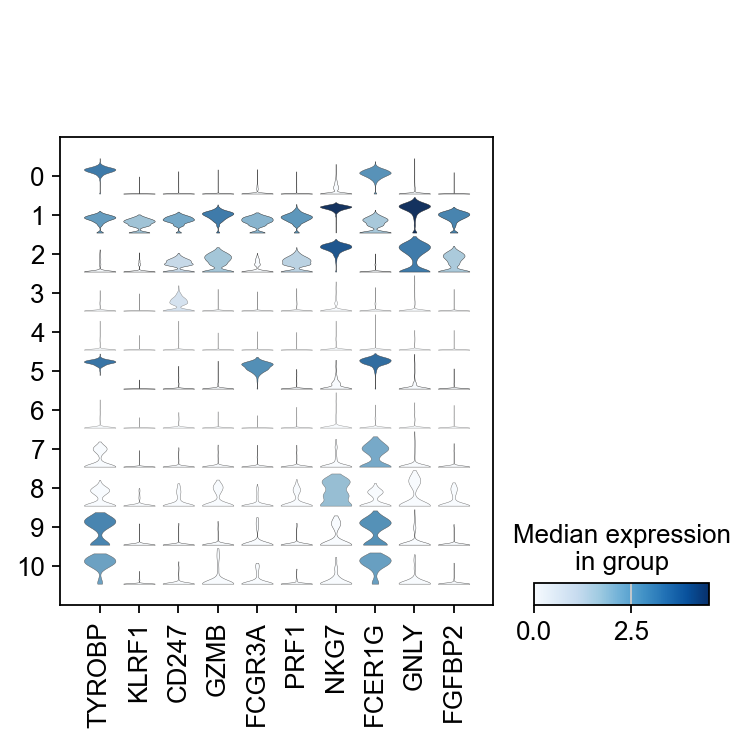
Plot as violins for those two groups, or across all the clusters.
sc.pl.rank_genes_groups_violin(adata, groups='1', n_genes=10)

# plot the same genes as violins across all the datasets.

# convert numpy.recarray to list
mynames = [x[0] for x in adata.uns['rank_genes_groups']['names'][:10]]
sc.pl.stacked_violin(adata, mynames, groupby = 'leiden_0.6')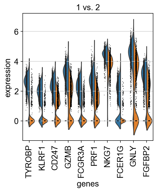
8 DGE across conditions
The second way of computing differential expression is to answer which genes are differentially expressed within a cluster. For example, in our case we have libraries comming from patients and controls and we would like to know which genes are influenced the most in a particular cell type. For this end, we will first subset our data for the desired cell cluster, then change the cell identities to the variable of comparison (which now in our case is the type, e.g. Covid/Ctrl).
cl1 = adata[adata.obs['leiden_0.6'] == '4',:]
cl1.obs['type'].value_counts()

sc.tl.rank_genes_groups(cl1, 'type', method='wilcoxon', key_added = "wilcoxon")
sc.pl.rank_genes_groups(cl1, n_genes=25, sharey=False, key="wilcoxon")
ranking genes
finished (0:00:01)
sc.pl.rank_genes_groups_violin(cl1, n_genes=10, key="wilcoxon")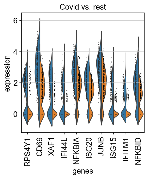
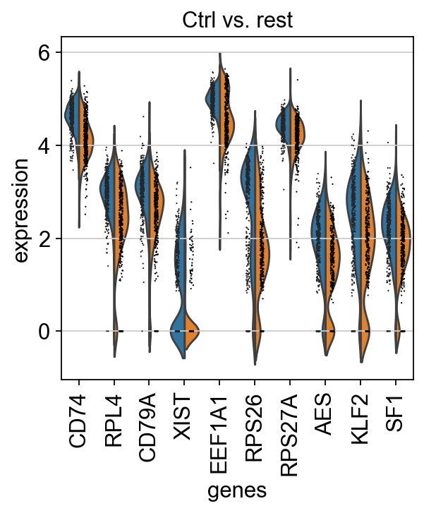
We can also plot these genes across all clusters, but split by “type”, to check if the genes are also up/downregulated in other celltypes.
import seaborn as sns

genes1 = sc.get.rank_genes_groups_df(cl1, group='Covid', key='wilcoxon')['names'][:5]
genes2 = sc.get.rank_genes_groups_df(cl1, group='Ctrl', key='wilcoxon')['names'][:5]
genes = genes1.tolist() +  genes2.tolist()
df = sc.get.obs_df(adata, genes + ['leiden_0.6','type'], use_raw=False)
df2 = df.melt(id_vars=["leiden_0.6",'type'], value_vars=genes)

sns.catplot(x = "leiden_0.6", y = "value", hue = "type", kind = 'violin', col = "variable", data = df2, col_wrap=4, inner=None)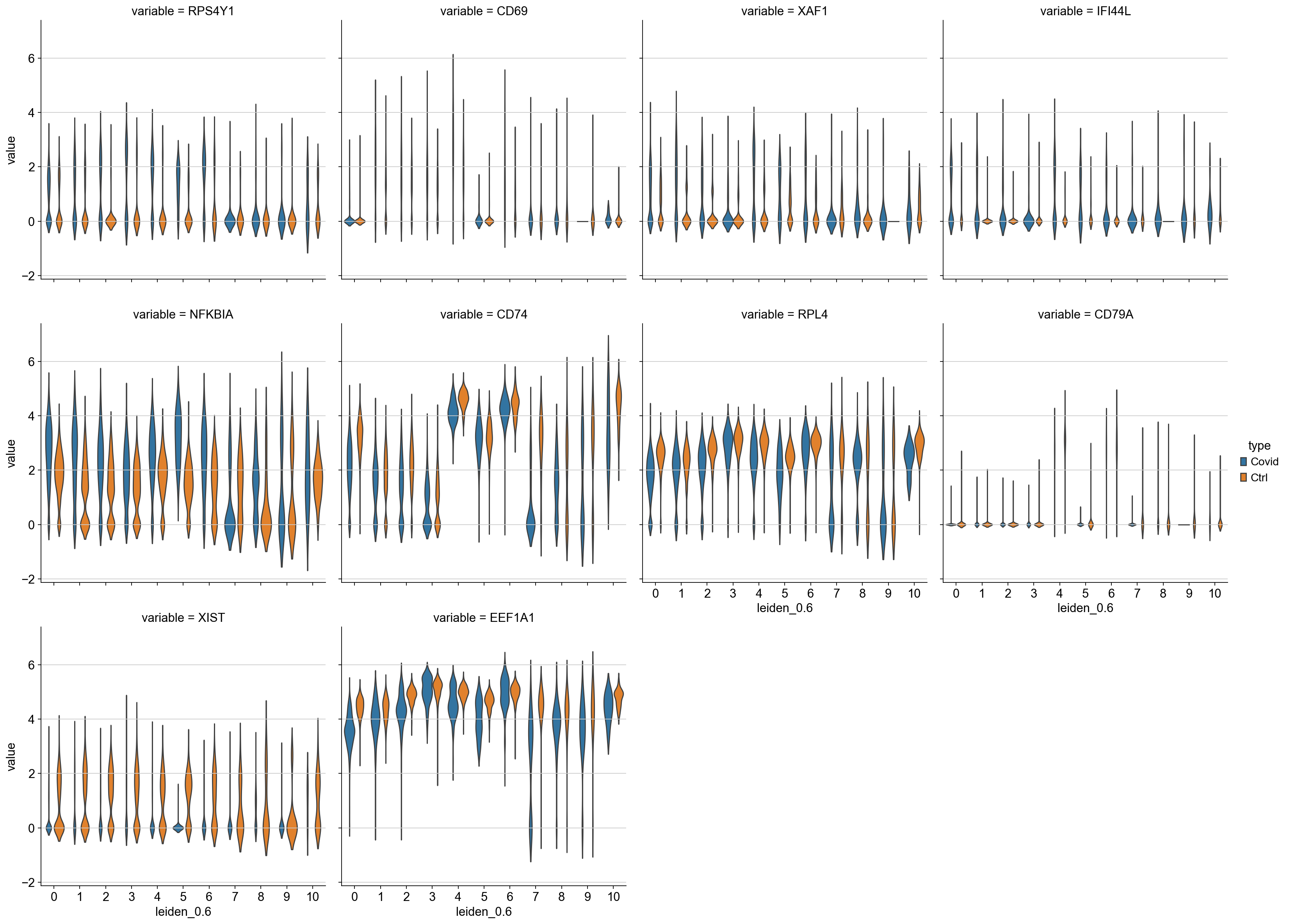
As you can see, we have many sex chromosome related genes among the top DE genes. And if you remember from the QC lab, we have inbalanced sex distribution among our subjects, so this is probably not related to covid at all.
8.1 Remove sex chromosome genes
To remove some of the bias due to inbalanced sex in the subjects we can remove the sex chromosome related genes.
annot_file = 'data/covid/results/gene_annotations_pybiomart.csv'

if not os.path.exists(annot_file):
    annot = sc.queries.biomart_annotations("hsapiens", ["ensembl_gene_id", "external_gene_name", "start_position", "end_position", "chromosome_name"] ).set_index("external_gene_name")
    annot.to_csv(annot_file)
else:
    annot = pd.read_csv(annot_file, index_col=0)

chrY_genes = adata.var_names.intersection(annot.index[annot.chromosome_name == "Y"])
chrX_genes = adata.var_names.intersection(annot.index[annot.chromosome_name == "X"])

sex_genes = chrY_genes.union(chrX_genes)
print(len(sex_genes))
all_genes = cl1.var.index.tolist()
print(len(all_genes))

keep_genes = [x for x in all_genes if x not in sex_genes]
print(len(keep_genes))

cl1 = cl1[:,keep_genes]
550
19468
18918Rerun differential expression.
sc.tl.rank_genes_groups(cl1, 'type', method='wilcoxon', key_added = "wilcoxon")
sc.pl.rank_genes_groups(cl1, n_genes=25, sharey=False, key="wilcoxon")
ranking genes
finished (0:00:01)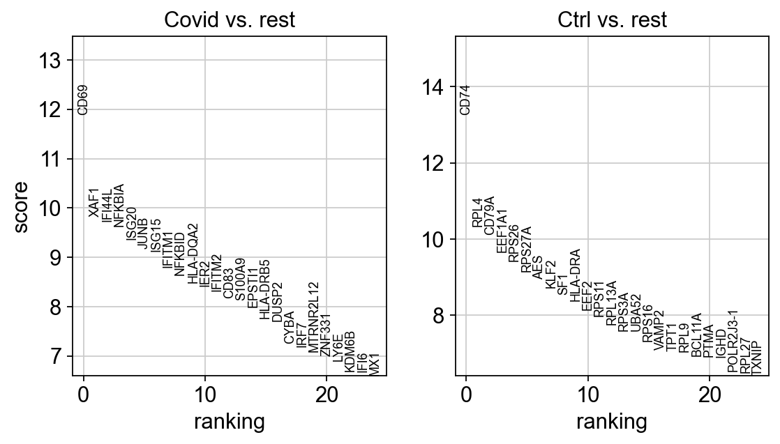
Now at least we do not have the sex chromosome genes as DE but still, some of the differences between patient and control could still be related to sex.
8.2 Patient batch effects
When we are testing for Covid vs Control we are running a DGE test for 4 vs 4 individuals. That will be very sensitive to sample differences unless we find a way to control for it. So first, lets check how the top DGEs are expressed in that cluster, across the individuals:
genes1 = sc.get.rank_genes_groups_df(cl1, group='Covid', key='wilcoxon')['names'][:5]
genes2 = sc.get.rank_genes_groups_df(cl1, group='Ctrl', key='wilcoxon')['names'][:5]
genes = genes1.tolist() +  genes2.tolist()

sc.pl.violin(cl1, genes1, groupby='sample', rotation=45)
sc.pl.violin(cl1, genes2, groupby='sample', rotation=45)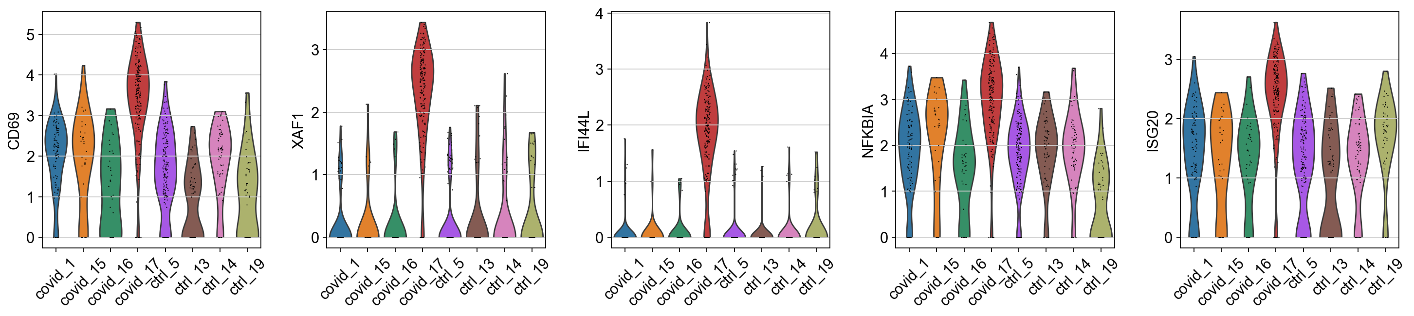
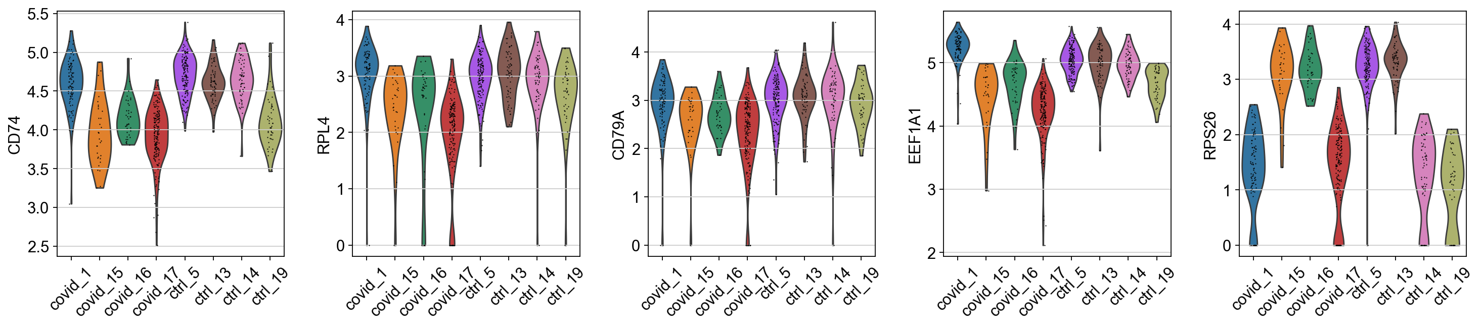
As you can see, many of the genes detected as DGE in Covid are unique to one or 2 patients.
We can also plot the top Covid and top Ctrl genes as a dotplot:
genes1 = sc.get.rank_genes_groups_df(cl1, group='Covid', key='wilcoxon')['names'][:20]
genes2 = sc.get.rank_genes_groups_df(cl1, group='Ctrl', key='wilcoxon')['names'][:20]
genes = genes1.tolist() +  genes2.tolist()

sc.pl.dotplot(cl1,genes, groupby='sample')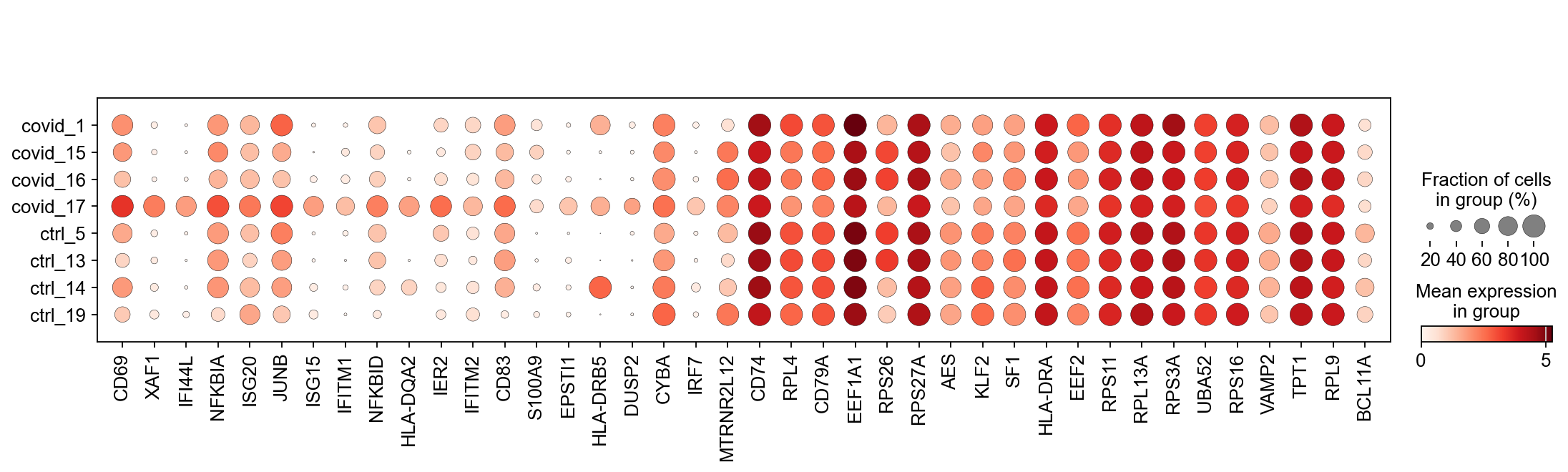
Clearly many of the top Covid genes are only high in the covid_17 sample, and not a general feature of covid patients.
This is also the patient with the highest number of cells in this cluster:
cl1.obs['sample'].value_counts()covid_17 207
ctrl_19 176
covid_1 136
ctrl_14 113
ctrl_13 112
covid_15 105
ctrl_5 43
covid_16 42
Name: sample, dtype: int648.3 Subsample
So one obvious thing to consider is an equal amount of cells per individual so that the DGE results are not dominated by a single sample.
So we will downsample to an equal number of cells per sample, in this case 34 cells per sample as it is the lowest number among all samples
target_cells = 37

tmp = [cl1[cl1.obs['sample'] == s] for s in cl1.obs['sample'].cat.categories]

for dat in tmp:
    if dat.n_obs > target_cells:
            sc.pp.subsample(dat, n_obs=target_cells)

cl1_sub = tmp[0].concatenate(*tmp[1:])

cl1_sub.obs['sample'].value_counts()
covid_1 37
covid_15 37
covid_16 37
covid_17 37
ctrl_5 37
ctrl_13 37
ctrl_14 37
ctrl_19 37
Name: sample, dtype: int64sc.tl.rank_genes_groups(cl1_sub, 'type', method='wilcoxon', key_added = "wilcoxon")
sc.pl.rank_genes_groups(cl1_sub, n_genes=25, sharey=False, key="wilcoxon")ranking genes
finished (0:00:00)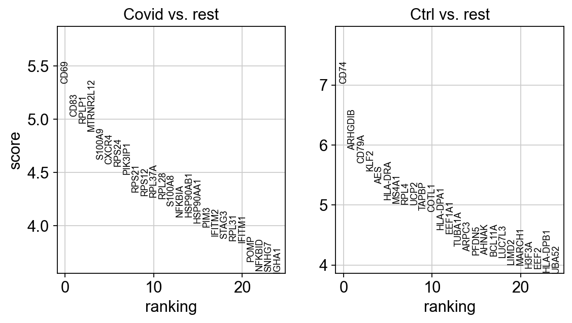
genes1 = sc.get.rank_genes_groups_df(cl1_sub, group='Covid', key='wilcoxon')['names'][:20]
genes2 = sc.get.rank_genes_groups_df(cl1_sub, group='Ctrl', key='wilcoxon')['names'][:20]
genes = genes1.tolist() +  genes2.tolist()

sc.pl.dotplot(cl1,genes, groupby='sample')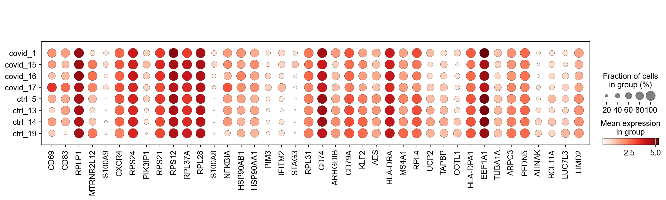
It looks much better now. But if we look per subject you can see that we still have some genes that are dominated by a single patient. Still, it is often a good idea to control the number of cells from each sample when doing differential expression.
There are many different ways to try and resolve the issue of patient batch effects, however most of them require R packages. These can be run via rpy2 as is demonstraded in this compendium: https://www.sc-best-practices.org/conditions/differential_gene_expression.html
However, we have not included it here as of now. So please have a look at the patient batch effect section in the seurat DGE tutorial where we run EdgeR on pseudobulk and MAST with random effect.
9 Gene Set Analysis (GSA)
9.1 Hypergeometric enrichment test
Having a defined list of differentially expressed genes, you can now look for their combined function using hypergeometric test.
#Available databases : ‘Human’, ‘Mouse’, ‘Yeast’, ‘Fly’, ‘Fish’, ‘Worm’
gene_set_names = gseapy.get_library_name(organism='Human')
print(gene_set_names)
['ARCHS4_Cell-lines', 'ARCHS4_IDG_Coexp', 'ARCHS4_Kinases_Coexp', 'ARCHS4_TFs_Coexp', 'ARCHS4_Tissues', 'Achilles_fitness_decrease', 'Achilles_fitness_increase', 'Aging_Perturbations_from_GEO_down', 'Aging_Perturbations_from_GEO_up', 'Allen_Brain_Atlas_10x_scRNA_2021', 'Allen_Brain_Atlas_down', 'Allen_Brain_Atlas_up', 'Azimuth_2023', 'Azimuth_Cell_Types_2021', 'BioCarta_2013', 'BioCarta_2015', 'BioCarta_2016', 'BioPlanet_2019', 'BioPlex_2017', 'CCLE_Proteomics_2020', 'CORUM', 'COVID-19_Related_Gene_Sets', 'COVID-19_Related_Gene_Sets_2021', 'Cancer_Cell_Line_Encyclopedia', 'CellMarker_2024', 'CellMarker_Augmented_2021', 'ChEA_2013', 'ChEA_2015', 'ChEA_2016', 'ChEA_2022', 'Chromosome_Location', 'Chromosome_Location_hg19', 'ClinVar_2019', 'DGIdb_Drug_Targets_2024', 'DSigDB', 'Data_Acquisition_Method_Most_Popular_Genes', 'DepMap_CRISPR_GeneDependency_CellLines_2023', 'DepMap_WG_CRISPR_Screens_Broad_CellLines_2019', 'DepMap_WG_CRISPR_Screens_Sanger_CellLines_2019', 'Descartes_Cell_Types_and_Tissue_2021', 'Diabetes_Perturbations_GEO_2022', 'DisGeNET', 'Disease_Perturbations_from_GEO_down', 'Disease_Perturbations_from_GEO_up', 'Disease_Signatures_from_GEO_down_2014', 'Disease_Signatures_from_GEO_up_2014', 'DrugMatrix', 'Drug_Perturbations_from_GEO_2014', 'Drug_Perturbations_from_GEO_down', 'Drug_Perturbations_from_GEO_up', 'ENCODE_Histone_Modifications_2013', 'ENCODE_Histone_Modifications_2015', 'ENCODE_TF_ChIP-seq_2014', 'ENCODE_TF_ChIP-seq_2015', 'ENCODE_and_ChEA_Consensus_TFs_from_ChIP-X', 'ESCAPE', 'Elsevier_Pathway_Collection', 'Enrichr_Libraries_Most_Popular_Genes', 'Enrichr_Submissions_TF-Gene_Coocurrence', 'Enrichr_Users_Contributed_Lists_2020', 'Epigenomics_Roadmap_HM_ChIP-seq', 'FANTOM6_lncRNA_KD_DEGs', 'GO_Biological_Process_2013', 'GO_Biological_Process_2015', 'GO_Biological_Process_2017', 'GO_Biological_Process_2017b', 'GO_Biological_Process_2018', 'GO_Biological_Process_2021', 'GO_Biological_Process_2023', 'GO_Cellular_Component_2013', 'GO_Cellular_Component_2015', 'GO_Cellular_Component_2017', 'GO_Cellular_Component_2017b', 'GO_Cellular_Component_2018', 'GO_Cellular_Component_2021', 'GO_Cellular_Component_2023', 'GO_Molecular_Function_2013', 'GO_Molecular_Function_2015', 'GO_Molecular_Function_2017', 'GO_Molecular_Function_2017b', 'GO_Molecular_Function_2018', 'GO_Molecular_Function_2021', 'GO_Molecular_Function_2023', 'GTEx_Aging_Signatures_2021', 'GTEx_Tissue_Expression_Down', 'GTEx_Tissue_Expression_Up', 'GTEx_Tissues_V8_2023', 'GWAS_Catalog_2019', 'GWAS_Catalog_2023', 'GeDiPNet_2023', 'GeneSigDB', 'Gene_Perturbations_from_GEO_down', 'Gene_Perturbations_from_GEO_up', 'Genes_Associated_with_NIH_Grants', 'Genome_Browser_PWMs', 'GlyGen_Glycosylated_Proteins_2022', 'HDSigDB_Human_2021', 'HDSigDB_Mouse_2021', 'HMDB_Metabolites', 'HMS_LINCS_KinomeScan', 'HomoloGene', 'HuBMAP_ASCT_plus_B_augmented_w_RNAseq_Coexpression', 'HuBMAP_ASCTplusB_augmented_2022', 'HumanCyc_2015', 'HumanCyc_2016', 'Human_Gene_Atlas', 'Human_Phenotype_Ontology', 'IDG_Drug_Targets_2022', 'InterPro_Domains_2019', 'Jensen_COMPARTMENTS', 'Jensen_DISEASES', 'Jensen_TISSUES', 'KEA_2013', 'KEA_2015', 'KEGG_2013', 'KEGG_2015', 'KEGG_2016', 'KEGG_2019_Human', 'KEGG_2019_Mouse', 'KEGG_2021_Human', 'KOMP2_Mouse_Phenotypes_2022', 'Kinase_Perturbations_from_GEO_down', 'Kinase_Perturbations_from_GEO_up', 'L1000_Kinase_and_GPCR_Perturbations_down', 'L1000_Kinase_and_GPCR_Perturbations_up', 'LINCS_L1000_CRISPR_KO_Consensus_Sigs', 'LINCS_L1000_Chem_Pert_Consensus_Sigs', 'LINCS_L1000_Chem_Pert_down', 'LINCS_L1000_Chem_Pert_up', 'LINCS_L1000_Ligand_Perturbations_down', 'LINCS_L1000_Ligand_Perturbations_up', 'Ligand_Perturbations_from_GEO_down', 'Ligand_Perturbations_from_GEO_up', 'MAGMA_Drugs_and_Diseases', 'MAGNET_2023', 'MCF7_Perturbations_from_GEO_down', 'MCF7_Perturbations_from_GEO_up', 'MGI_Mammalian_Phenotype_2013', 'MGI_Mammalian_Phenotype_2017', 'MGI_Mammalian_Phenotype_Level_3', 'MGI_Mammalian_Phenotype_Level_4', 'MGI_Mammalian_Phenotype_Level_4_2019', 'MGI_Mammalian_Phenotype_Level_4_2021', 'MGI_Mammalian_Phenotype_Level_4_2024', 'MSigDB_Computational', 'MSigDB_Hallmark_2020', 'MSigDB_Oncogenic_Signatures', 'Metabolomics_Workbench_Metabolites_2022', 'Microbe_Perturbations_from_GEO_down', 'Microbe_Perturbations_from_GEO_up', 'MoTrPAC_2023', 'Mouse_Gene_Atlas', 'NCI-60_Cancer_Cell_Lines', 'NCI-Nature_2016', 'NIH_Funded_PIs_2017_AutoRIF_ARCHS4_Predictions', 'NIH_Funded_PIs_2017_GeneRIF_ARCHS4_Predictions', 'NIH_Funded_PIs_2017_Human_AutoRIF', 'NIH_Funded_PIs_2017_Human_GeneRIF', 'NURSA_Human_Endogenous_Complexome', 'OMIM_Disease', 'OMIM_Expanded', 'Old_CMAP_down', 'Old_CMAP_up', 'Orphanet_Augmented_2021', 'PFOCR_Pathways', 'PFOCR_Pathways_2023', 'PPI_Hub_Proteins', 'PanglaoDB_Augmented_2021', 'Panther_2015', 'Panther_2016', 'PerturbAtlas', 'Pfam_Domains_2019', 'Pfam_InterPro_Domains', 'PheWeb_2019', 'PhenGenI_Association_2021', 'Phosphatase_Substrates_from_DEPOD', 'ProteomicsDB_2020', 'Proteomics_Drug_Atlas_2023', 'RNA-Seq_Disease_Gene_and_Drug_Signatures_from_GEO', 'RNAseq_Automatic_GEO_Signatures_Human_Down', 'RNAseq_Automatic_GEO_Signatures_Human_Up', 'RNAseq_Automatic_GEO_Signatures_Mouse_Down', 'RNAseq_Automatic_GEO_Signatures_Mouse_Up', 'Rare_Diseases_AutoRIF_ARCHS4_Predictions', 'Rare_Diseases_AutoRIF_Gene_Lists', 'Rare_Diseases_GeneRIF_ARCHS4_Predictions', 'Rare_Diseases_GeneRIF_Gene_Lists', 'Reactome_2013', 'Reactome_2015', 'Reactome_2016', 'Reactome_2022', 'Reactome_Pathways_2024', 'Rummagene_kinases', 'Rummagene_signatures', 'Rummagene_transcription_factors', 'SILAC_Phosphoproteomics', 'SubCell_BarCode', 'SynGO_2022', 'SynGO_2024', 'SysMyo_Muscle_Gene_Sets', 'TF-LOF_Expression_from_GEO', 'TF_Perturbations_Followed_by_Expression', 'TG_GATES_2020', 'TRANSFAC_and_JASPAR_PWMs', 'TRRUST_Transcription_Factors_2019', 'Table_Mining_of_CRISPR_Studies', 'Tabula_Muris', 'Tabula_Sapiens', 'TargetScan_microRNA', 'TargetScan_microRNA_2017', 'The_Kinase_Library_2023', 'The_Kinase_Library_2024', 'Tissue_Protein_Expression_from_Human_Proteome_Map', 'Tissue_Protein_Expression_from_ProteomicsDB', 'Transcription_Factor_PPIs', 'UK_Biobank_GWAS_v1', 'Virus-Host_PPI_P-HIPSTer_2020', 'VirusMINT', 'Virus_Perturbations_from_GEO_down', 'Virus_Perturbations_from_GEO_up', 'WikiPathway_2021_Human', 'WikiPathway_2023_Human', 'WikiPathways_2013', 'WikiPathways_2015', 'WikiPathways_2016', 'WikiPathways_2019_Human', 'WikiPathways_2019_Mouse', 'WikiPathways_2024_Human', 'WikiPathways_2024_Mouse', 'dbGaP', 'huMAP', 'lncHUB_lncRNA_Co-Expression', 'miRTarBase_2017']Get the significant DEGs for the Covid patients.
#?gseapy.enrichr
glist = sc.get.rank_genes_groups_df(cl1_sub, group='Covid', key='wilcoxon', log2fc_min=0.25, pval_cutoff=0.05)['names'].squeeze().str.strip().tolist()
print(len(glist))457enr_res = gseapy.enrichr(gene_list=glist, organism='Human', gene_sets='GO_Biological_Process_2018', cutoff = 0.5)
enr_res.results.head()| Gene_set | Term | Overlap | P-value | Adjusted P-value | Old P-value | Old Adjusted P-value | Odds Ratio | Combined Score | Genes | |
|---|---|---|---|---|---|---|---|---|---|---|
| 0 | GO_Biological_Process_2018 | neutrophil degranulation (GO:0043312) | 74/479 | 5.480891e-40 | 1.192287e-36 | 0 | 0 | 9.130078 | 825.378525 | CDA;ITGAM;TNFAIP6;SLC2A3;PYGL;PYCARD;HK3;GM2A;... |
| 1 | GO_Biological_Process_2018 | neutrophil activation involved in immune respo... | 74/483 | 9.882200e-40 | 1.192287e-36 | 0 | 0 | 9.038896 | 811.807404 | CDA;ITGAM;TNFAIP6;SLC2A3;PYGL;PYCARD;HK3;GM2A;... |
| 2 | GO_Biological_Process_2018 | neutrophil mediated immunity (GO:0002446) | 74/487 | 1.771138e-39 | 1.424585e-36 | 0 | 0 | 8.949481 | 798.555025 | CDA;ITGAM;TNFAIP6;SLC2A3;PYGL;PYCARD;HK3;GM2A;... |
| 3 | GO_Biological_Process_2018 | cytokine-mediated signaling pathway (GO:0019221) | 49/633 | 8.185037e-14 | 4.937623e-11 | 0 | 0 | 3.898868 | 117.488025 | ITGAM;IFITM2;CXCL8;IRS2;IL1RAP;IFI35;TXNDC17;L... |
| 4 | GO_Biological_Process_2018 | response to lipopolysaccharide (GO:0032496) | 21/155 | 6.106515e-11 | 2.947004e-08 | 0 | 0 | 6.976397 | 164.078430 | JUN;CXCL8;SLC11A1;HMGB2;LY96;TNFAIP3;IRAK3;PPB... |
Some databases of interest:
GO_Biological_Process_2017bKEGG_2019_HumanKEGG_2019_MouseWikiPathways_2019_HumanWikiPathways_2019_Mouse
You visualize your results using a simple barplot, for example:
gseapy.barplot(enr_res.res2d,title='GO_Biological_Process_2018')<Axes: title={'center': 'GO_Biological_Process_2018'}, xlabel='$- \\log_{10}$ (Adjusted P-value)'>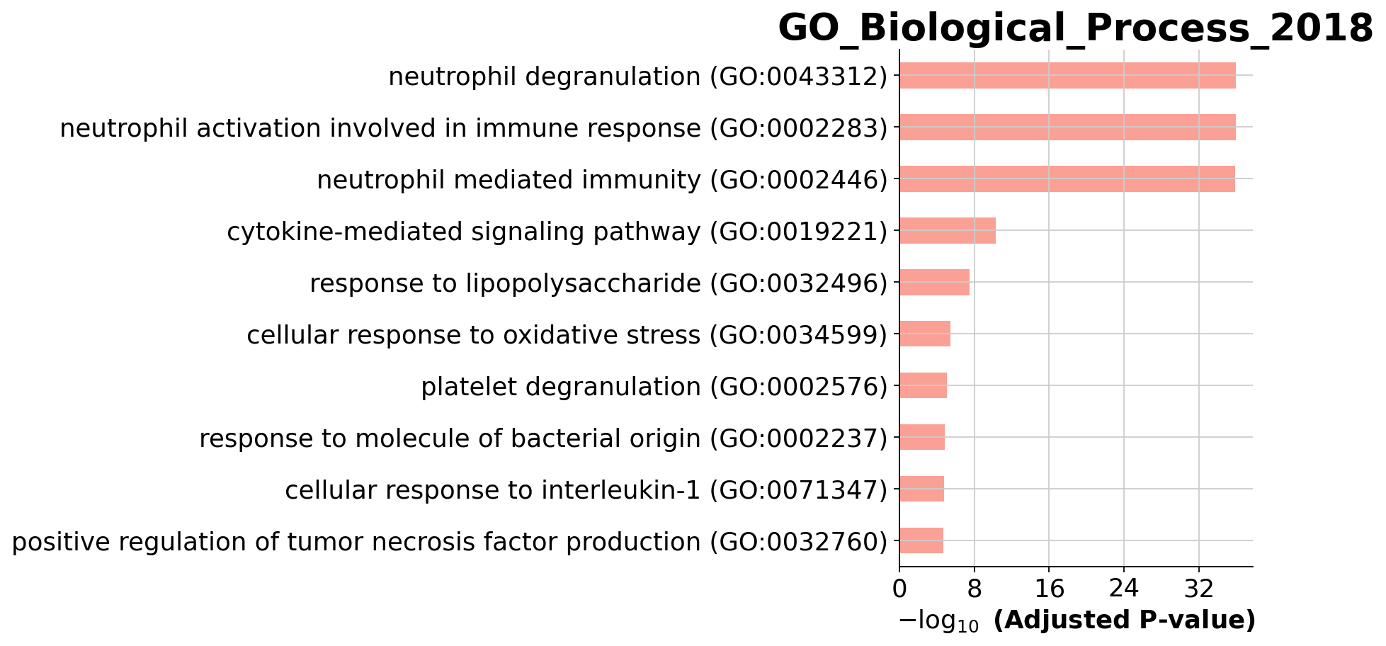
10 Gene Set Enrichment Analysis (GSEA)
Besides the enrichment using hypergeometric test, we can also perform gene set enrichment analysis (GSEA), which scores ranked genes list (usually based on fold changes) and computes permutation test to check if a particular gene set is more present in the Up-regulated genes, among the DOWN_regulated genes or not differentially regulated.
We need a table with all DEGs and their log foldchanges. However, many lowly expressed genes will have high foldchanges and just contribue noise, so also filter for expression in enough cells.
gene_rank = sc.get.rank_genes_groups_df(cl1_sub, group='Covid', key='wilcoxon')[['names','logfoldchanges']]
gene_rank.sort_values(by=['logfoldchanges'], inplace=True, ascending=False)

# calculate_qc_metrics will calculate number of cells per gene
sc.pp.calculate_qc_metrics(cl1, percent_top=None, log1p=False, inplace=True)

# filter for genes expressed in at least 30 cells.
gene_rank = gene_rank[gene_rank['names'].isin(cl1.var_names[cl1.var.n_cells_by_counts>30])]

gene_rank| names | logfoldchanges | |
|---|---|---|
| 180 | SERPINB2 | 29.298830 |
| 119 | MTRNR2L1 | 29.095734 |
| 315 | ADAMTS2 | 28.207029 |
| 858 | CLEC1B | 27.513737 |
| 922 | IGLC3 | 27.425417 |
| ... | ... | ... |
| 15550 | ATP1B1 | -24.515152 |
| 17157 | BTBD11 | -25.881178 |
| 17716 | AFF3 | -26.617949 |
| 18086 | PLD4 | -27.048063 |
| 18648 | AC004556.1 | -28.077997 |
9604 rows × 2 columns
Once our list of genes are sorted, we can proceed with the enrichment itself. We can use the package to get gene set from the Molecular Signature Database (MSigDB) and select KEGG pathways as an example.
#Available databases : ‘Human’, ‘Mouse’, ‘Yeast’, ‘Fly’, ‘Fish’, ‘Worm’
gene_set_names = gseapy.get_library_name(organism='Human')
print(gene_set_names)
['ARCHS4_Cell-lines', 'ARCHS4_IDG_Coexp', 'ARCHS4_Kinases_Coexp', 'ARCHS4_TFs_Coexp', 'ARCHS4_Tissues', 'Achilles_fitness_decrease', 'Achilles_fitness_increase', 'Aging_Perturbations_from_GEO_down', 'Aging_Perturbations_from_GEO_up', 'Allen_Brain_Atlas_10x_scRNA_2021', 'Allen_Brain_Atlas_down', 'Allen_Brain_Atlas_up', 'Azimuth_2023', 'Azimuth_Cell_Types_2021', 'BioCarta_2013', 'BioCarta_2015', 'BioCarta_2016', 'BioPlanet_2019', 'BioPlex_2017', 'CCLE_Proteomics_2020', 'CORUM', 'COVID-19_Related_Gene_Sets', 'COVID-19_Related_Gene_Sets_2021', 'Cancer_Cell_Line_Encyclopedia', 'CellMarker_2024', 'CellMarker_Augmented_2021', 'ChEA_2013', 'ChEA_2015', 'ChEA_2016', 'ChEA_2022', 'Chromosome_Location', 'Chromosome_Location_hg19', 'ClinVar_2019', 'DGIdb_Drug_Targets_2024', 'DSigDB', 'Data_Acquisition_Method_Most_Popular_Genes', 'DepMap_CRISPR_GeneDependency_CellLines_2023', 'DepMap_WG_CRISPR_Screens_Broad_CellLines_2019', 'DepMap_WG_CRISPR_Screens_Sanger_CellLines_2019', 'Descartes_Cell_Types_and_Tissue_2021', 'Diabetes_Perturbations_GEO_2022', 'DisGeNET', 'Disease_Perturbations_from_GEO_down', 'Disease_Perturbations_from_GEO_up', 'Disease_Signatures_from_GEO_down_2014', 'Disease_Signatures_from_GEO_up_2014', 'DrugMatrix', 'Drug_Perturbations_from_GEO_2014', 'Drug_Perturbations_from_GEO_down', 'Drug_Perturbations_from_GEO_up', 'ENCODE_Histone_Modifications_2013', 'ENCODE_Histone_Modifications_2015', 'ENCODE_TF_ChIP-seq_2014', 'ENCODE_TF_ChIP-seq_2015', 'ENCODE_and_ChEA_Consensus_TFs_from_ChIP-X', 'ESCAPE', 'Elsevier_Pathway_Collection', 'Enrichr_Libraries_Most_Popular_Genes', 'Enrichr_Submissions_TF-Gene_Coocurrence', 'Enrichr_Users_Contributed_Lists_2020', 'Epigenomics_Roadmap_HM_ChIP-seq', 'FANTOM6_lncRNA_KD_DEGs', 'GO_Biological_Process_2013', 'GO_Biological_Process_2015', 'GO_Biological_Process_2017', 'GO_Biological_Process_2017b', 'GO_Biological_Process_2018', 'GO_Biological_Process_2021', 'GO_Biological_Process_2023', 'GO_Cellular_Component_2013', 'GO_Cellular_Component_2015', 'GO_Cellular_Component_2017', 'GO_Cellular_Component_2017b', 'GO_Cellular_Component_2018', 'GO_Cellular_Component_2021', 'GO_Cellular_Component_2023', 'GO_Molecular_Function_2013', 'GO_Molecular_Function_2015', 'GO_Molecular_Function_2017', 'GO_Molecular_Function_2017b', 'GO_Molecular_Function_2018', 'GO_Molecular_Function_2021', 'GO_Molecular_Function_2023', 'GTEx_Aging_Signatures_2021', 'GTEx_Tissue_Expression_Down', 'GTEx_Tissue_Expression_Up', 'GTEx_Tissues_V8_2023', 'GWAS_Catalog_2019', 'GWAS_Catalog_2023', 'GeDiPNet_2023', 'GeneSigDB', 'Gene_Perturbations_from_GEO_down', 'Gene_Perturbations_from_GEO_up', 'Genes_Associated_with_NIH_Grants', 'Genome_Browser_PWMs', 'GlyGen_Glycosylated_Proteins_2022', 'HDSigDB_Human_2021', 'HDSigDB_Mouse_2021', 'HMDB_Metabolites', 'HMS_LINCS_KinomeScan', 'HomoloGene', 'HuBMAP_ASCT_plus_B_augmented_w_RNAseq_Coexpression', 'HuBMAP_ASCTplusB_augmented_2022', 'HumanCyc_2015', 'HumanCyc_2016', 'Human_Gene_Atlas', 'Human_Phenotype_Ontology', 'IDG_Drug_Targets_2022', 'InterPro_Domains_2019', 'Jensen_COMPARTMENTS', 'Jensen_DISEASES', 'Jensen_TISSUES', 'KEA_2013', 'KEA_2015', 'KEGG_2013', 'KEGG_2015', 'KEGG_2016', 'KEGG_2019_Human', 'KEGG_2019_Mouse', 'KEGG_2021_Human', 'KOMP2_Mouse_Phenotypes_2022', 'Kinase_Perturbations_from_GEO_down', 'Kinase_Perturbations_from_GEO_up', 'L1000_Kinase_and_GPCR_Perturbations_down', 'L1000_Kinase_and_GPCR_Perturbations_up', 'LINCS_L1000_CRISPR_KO_Consensus_Sigs', 'LINCS_L1000_Chem_Pert_Consensus_Sigs', 'LINCS_L1000_Chem_Pert_down', 'LINCS_L1000_Chem_Pert_up', 'LINCS_L1000_Ligand_Perturbations_down', 'LINCS_L1000_Ligand_Perturbations_up', 'Ligand_Perturbations_from_GEO_down', 'Ligand_Perturbations_from_GEO_up', 'MAGMA_Drugs_and_Diseases', 'MAGNET_2023', 'MCF7_Perturbations_from_GEO_down', 'MCF7_Perturbations_from_GEO_up', 'MGI_Mammalian_Phenotype_2013', 'MGI_Mammalian_Phenotype_2017', 'MGI_Mammalian_Phenotype_Level_3', 'MGI_Mammalian_Phenotype_Level_4', 'MGI_Mammalian_Phenotype_Level_4_2019', 'MGI_Mammalian_Phenotype_Level_4_2021', 'MGI_Mammalian_Phenotype_Level_4_2024', 'MSigDB_Computational', 'MSigDB_Hallmark_2020', 'MSigDB_Oncogenic_Signatures', 'Metabolomics_Workbench_Metabolites_2022', 'Microbe_Perturbations_from_GEO_down', 'Microbe_Perturbations_from_GEO_up', 'MoTrPAC_2023', 'Mouse_Gene_Atlas', 'NCI-60_Cancer_Cell_Lines', 'NCI-Nature_2016', 'NIH_Funded_PIs_2017_AutoRIF_ARCHS4_Predictions', 'NIH_Funded_PIs_2017_GeneRIF_ARCHS4_Predictions', 'NIH_Funded_PIs_2017_Human_AutoRIF', 'NIH_Funded_PIs_2017_Human_GeneRIF', 'NURSA_Human_Endogenous_Complexome', 'OMIM_Disease', 'OMIM_Expanded', 'Old_CMAP_down', 'Old_CMAP_up', 'Orphanet_Augmented_2021', 'PFOCR_Pathways', 'PFOCR_Pathways_2023', 'PPI_Hub_Proteins', 'PanglaoDB_Augmented_2021', 'Panther_2015', 'Panther_2016', 'PerturbAtlas', 'Pfam_Domains_2019', 'Pfam_InterPro_Domains', 'PheWeb_2019', 'PhenGenI_Association_2021', 'Phosphatase_Substrates_from_DEPOD', 'ProteomicsDB_2020', 'Proteomics_Drug_Atlas_2023', 'RNA-Seq_Disease_Gene_and_Drug_Signatures_from_GEO', 'RNAseq_Automatic_GEO_Signatures_Human_Down', 'RNAseq_Automatic_GEO_Signatures_Human_Up', 'RNAseq_Automatic_GEO_Signatures_Mouse_Down', 'RNAseq_Automatic_GEO_Signatures_Mouse_Up', 'Rare_Diseases_AutoRIF_ARCHS4_Predictions', 'Rare_Diseases_AutoRIF_Gene_Lists', 'Rare_Diseases_GeneRIF_ARCHS4_Predictions', 'Rare_Diseases_GeneRIF_Gene_Lists', 'Reactome_2013', 'Reactome_2015', 'Reactome_2016', 'Reactome_2022', 'Reactome_Pathways_2024', 'Rummagene_kinases', 'Rummagene_signatures', 'Rummagene_transcription_factors', 'SILAC_Phosphoproteomics', 'SubCell_BarCode', 'SynGO_2022', 'SynGO_2024', 'SysMyo_Muscle_Gene_Sets', 'TF-LOF_Expression_from_GEO', 'TF_Perturbations_Followed_by_Expression', 'TG_GATES_2020', 'TRANSFAC_and_JASPAR_PWMs', 'TRRUST_Transcription_Factors_2019', 'Table_Mining_of_CRISPR_Studies', 'Tabula_Muris', 'Tabula_Sapiens', 'TargetScan_microRNA', 'TargetScan_microRNA_2017', 'The_Kinase_Library_2023', 'The_Kinase_Library_2024', 'Tissue_Protein_Expression_from_Human_Proteome_Map', 'Tissue_Protein_Expression_from_ProteomicsDB', 'Transcription_Factor_PPIs', 'UK_Biobank_GWAS_v1', 'Virus-Host_PPI_P-HIPSTer_2020', 'VirusMINT', 'Virus_Perturbations_from_GEO_down', 'Virus_Perturbations_from_GEO_up', 'WikiPathway_2021_Human', 'WikiPathway_2023_Human', 'WikiPathways_2013', 'WikiPathways_2015', 'WikiPathways_2016', 'WikiPathways_2019_Human', 'WikiPathways_2019_Mouse', 'WikiPathways_2024_Human', 'WikiPathways_2024_Mouse', 'dbGaP', 'huMAP', 'lncHUB_lncRNA_Co-Expression', 'miRTarBase_2017']Next, we will run GSEA. This will result in a table containing information for several pathways. We can then sort and filter those pathways to visualize only the top ones. You can select/filter them by either p-value or normalized enrichment score (NES).
res = gseapy.prerank(rnk=gene_rank, gene_sets='KEGG_2021_Human')

terms = res.res2d.Term
terms[:10]
0 Cardiac muscle contraction
1 Endocrine and other factor-regulated calcium r...
2 Carbohydrate digestion and absorption
3 Viral protein interaction with cytokine and cy...
4 Ether lipid metabolism
5 Protein digestion and absorption
6 Malaria
7 Aldosterone-regulated sodium reabsorption
8 Primary immunodeficiency
9 Mineral absorption
Name: Term, dtype: objectgseapy.gseaplot(rank_metric=res.ranking, term=terms[0], **res.results[terms[0]])[<Axes: xlabel='Gene Rank', ylabel='Ranked metric'>,
<Axes: >,
<Axes: >,
<Axes: ylabel='Enrichment Score'>]![]()
Discuss
Which KEGG pathways are upregulated in this cluster? Which KEGG pathways are dowregulated in this cluster? Change the pathway source to another gene set (e.g. CP:WIKIPATHWAYS or CP:REACTOME or CP:BIOCARTA or GO:BP) and check the if you get similar results?
Finally, let’s save the integrated data for further analysis.
adata.write_h5ad('./data/covid/results/scanpy_covid_qc_dr_scanorama_cl_dge.h5ad')11 Session info
Click here
sc.logging.print_versions()-----
anndata 0.10.8
scanpy 1.10.3
-----
PIL 11.1.0
asttokens NA
brotli 1.1.0
certifi 2024.12.14
cffi 1.17.1
charset_normalizer 3.4.1
colorama 0.4.6
comm 0.2.2
cycler 0.12.1
cython_runtime NA
dateutil 2.9.0.post0
debugpy 1.8.12
decorator 5.1.1
exceptiongroup 1.2.2
executing 2.1.0
gseapy 1.1.3
h5py 3.12.1
idna 3.10
igraph 0.11.6
ipykernel 6.29.5
jedi 0.19.2
joblib 1.4.2
kiwisolver 1.4.7
legacy_api_wrap NA
leidenalg 0.10.2
llvmlite 0.43.0
matplotlib 3.9.2
matplotlib_inline 0.1.7
matplotlib_venn 1.1.1
mpl_toolkits NA
natsort 8.4.0
numba 0.60.0
numpy 1.26.4
packaging 24.2
pandas 1.5.3
parso 0.8.4
patsy 1.0.1
pickleshare 0.7.5
platformdirs 4.3.6
prompt_toolkit 3.0.50
psutil 6.1.1
pure_eval 0.2.3
pycparser 2.22
pydev_ipython NA
pydevconsole NA
pydevd 3.2.3
pydevd_file_utils NA
pydevd_plugins NA
pydevd_tracing NA
pygments 2.19.1
pyparsing 3.2.1
pytz 2024.2
requests 2.32.3
scipy 1.14.1
seaborn 0.13.2
session_info 1.0.0
six 1.17.0
sklearn 1.6.1
socks 1.7.1
sparse 0.15.5
stack_data 0.6.3
statsmodels 0.14.4
texttable 1.7.0
threadpoolctl 3.5.0
torch 2.5.1.post207
torchgen NA
tornado 6.4.2
tqdm 4.67.1
traitlets 5.14.3
typing_extensions NA
urllib3 2.3.0
wcwidth 0.2.13
yaml 6.0.2
zmq 26.2.0
zoneinfo NA
zstandard 0.23.0
-----
IPython 8.31.0
jupyter_client 8.6.3
jupyter_core 5.7.2
-----
Python 3.10.16 | packaged by conda-forge | (main, Dec 5 2024, 14:16:10) [GCC 13.3.0]
Linux-6.10.14-linuxkit-x86_64-with-glibc2.35
-----
Session information updated at 2025-02-27 15:23