import numpy as np
import pandas as pd
import scanpy as sc
import matplotlib.pyplot as plt
import warnings
import os
import subprocess

warnings.simplefilter(action="ignore", category=Warning)

# verbosity: errors (0), warnings (1), info (2), hints (3)
sc.settings.verbosity = 3
sc.settings.set_figure_params(dpi=80)
Note
Code chunks run Python commands unless it starts with %%bash, in which case, those chunks run shell commands.
In this tutorial we will continue the analysis of the integrated dataset. We will use the scanpy enbedding to perform the clustering using graph community detection algorithms.
Let’s first load all necessary libraries and also the integrated dataset from the previous step.
# download pre-computed data if missing or long compute
fetch_data = True

# url for source and intermediate data
path_data = "https://nextcloud.dc.scilifelab.se/public.php/webdav"
curl_upass = "zbC5fr2LbEZ9rSE:scRNAseq2025"

path_results = "data/covid/results"
if not os.path.exists(path_results):
    os.makedirs(path_results, exist_ok=True)

path_file = "data/covid/results/scanpy_covid_qc_dr_int.h5ad"
if fetch_data and not os.path.exists(path_file):
    file_url = os.path.join(path_data, "covid/results_scanpy/scanpy_covid_qc_dr_int.h5ad")
    subprocess.call(["curl", "-u", curl_upass, "-o", path_file, file_url ])

adata = sc.read_h5ad(path_file)
adata
AnnData object with n_obs × n_vars = 7332 × 19468
obs: 'type', 'sample', 'batch', 'n_genes_by_counts', 'total_counts', 'total_counts_mt', 'pct_counts_mt', 'total_counts_ribo', 'pct_counts_ribo', 'total_counts_hb', 'pct_counts_hb', 'percent_mt2', 'n_counts', 'n_genes', 'percent_chrY', 'XIST-counts', 'S_score', 'G2M_score', 'phase', 'doublet_scores', 'predicted_doublets', 'doublet_info', 'leiden'
var: 'gene_ids', 'feature_types', 'genome', 'mt', 'ribo', 'hb', 'n_cells_by_counts', 'mean_counts', 'pct_dropout_by_counts', 'total_counts', 'n_cells', 'highly_variable', 'means', 'dispersions', 'dispersions_norm', 'highly_variable_nbatches', 'highly_variable_intersection'
uns: 'doublet_info_colors', 'hvg', 'leiden', 'log1p', 'neighbors', 'pca', 'phase_colors', 'sample_colors', 'tsne', 'umap'
obsm: 'Scanorama', 'X_pca', 'X_pca_harmony', 'X_tsne', 'X_tsne_bbknn', 'X_tsne_harmony', 'X_tsne_scanorama', 'X_tsne_uncorr', 'X_umap', 'X_umap_bbknn', 'X_umap_harmony', 'X_umap_scanorama', 'X_umap_uncorr'
obsp: 'connectivities', 'distances'1 Graph clustering
The procedure of clustering on a Graph can be generalized as 3 main steps:
- Build a kNN graph from the data.
- Prune spurious connections from kNN graph (optional step). This is a SNN graph.
- Find groups of cells that maximizes the connections within the group compared other groups.
In Scanpy we do not build an SNN graph, instead the community detection is done on the KNN graph which we construct using the command sc.pp.neighbors().
The main options to consider are:
- n_pcs - the number of dimensions from the initial reduction to include when calculating distances between cells.
- n_neighbors - the number of neighbors per cell to include in the KNN graph.
In this case, we will use the integrated data using Harmony. If you recall, we stored the harmony reduction in X_pca_harmony in the previous lab.
sc.pp.neighbors(adata, n_neighbors=20, n_pcs=30, use_rep='X_pca_harmony')

# We will also set the default umap to the one created with harmony
# so that sc.pl.umap selects that embedding.
adata.obsm["X_umap"] = adata.obsm["X_umap_harmony"]
computing neighbors
finished: added to `.uns['neighbors']`
`.obsp['distances']`, distances for each pair of neighbors
`.obsp['connectivities']`, weighted adjacency matrix (0:00:10)The modularity optimization algoritm in Scanpy is Leiden. Previously ther was also Louvain, but since the Louvain algorithm is no longer maintained, using Leiden is recommended by the Scanpy community.
1.1 Leiden
# default resolution is 1.0, but we will try a few different values.
sc.tl.leiden(adata, resolution = 0.4, key_added = "leiden_0.4")
sc.tl.leiden(adata, resolution = 0.6, key_added = "leiden_0.6")
sc.tl.leiden(adata, resolution = 1.0, key_added = "leiden_1.0")
sc.tl.leiden(adata, resolution = 1.4, key_added = "leiden_1.4")
running Leiden clustering
finished: found 10 clusters and added
'leiden_0.4', the cluster labels (adata.obs, categorical) (0:00:00)
running Leiden clustering
finished: found 11 clusters and added
'leiden_0.6', the cluster labels (adata.obs, categorical) (0:00:00)
running Leiden clustering
finished: found 16 clusters and added
'leiden_1.0', the cluster labels (adata.obs, categorical) (0:00:00)
running Leiden clustering
finished: found 19 clusters and added
'leiden_1.4', the cluster labels (adata.obs, categorical) (0:00:00)Plot the clusters, as you can see, with increased resolution, we get higher granularity in the clustering.
sc.pl.umap(adata, color=['leiden_0.4', 'leiden_0.6', 'leiden_1.0','leiden_1.4'], legend_fontsize=8)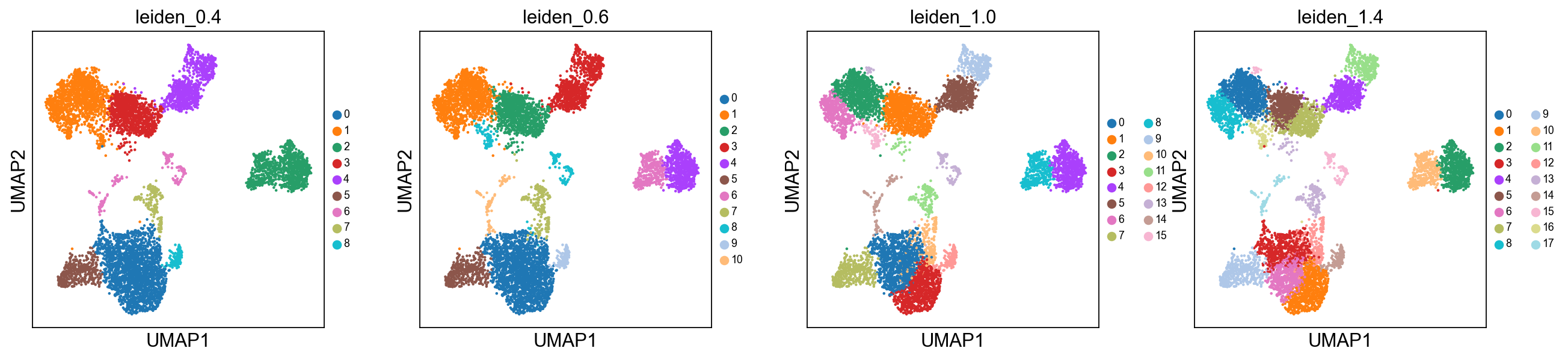
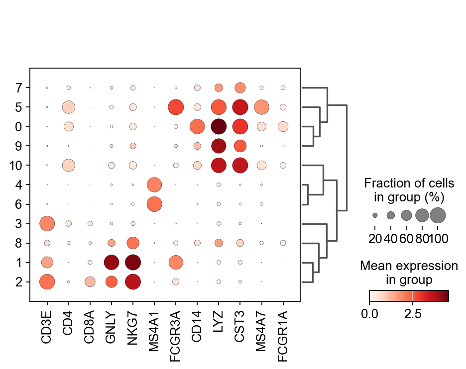
Once we have done clustering, the relationships between clusters can be calculated as correlation in PCA space and we also visualize some of the marker genes that we used in the Dim Reduction lab onto the clusters. If we set dendrogram=True the clusters are ordered by the dendrogram in the dotplot.
sc.tl.dendrogram(adata, groupby = "leiden_0.6")
sc.pl.dendrogram(adata, groupby = "leiden_0.6")

genes  = ["CD3E", "CD4", "CD8A", "GNLY","NKG7", "MS4A1","FCGR3A","CD14","LYZ","CST3","MS4A7","FCGR1A"]
sc.pl.dotplot(adata, genes, groupby='leiden_0.6', dendrogram=True)
using 'X_pca' with n_pcs = 50
Storing dendrogram info using `.uns['dendrogram_leiden_0.6']`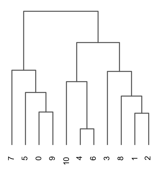
2 K-means clustering
K-means is a generic clustering algorithm that has been used in many application areas. In R, it can be applied via the kmeans() function. Typically, it is applied to a reduced dimension representation of the expression data (most often PCA, because of the interpretability of the low-dimensional distances). We need to define the number of clusters in advance. Since the results depend on the initialization of the cluster centers, it is typically recommended to run K-means with multiple starting configurations (via the nstart argument).
from sklearn.cluster import KMeans
from sklearn.metrics import adjusted_rand_score

# extract pca coordinates
X_pca = adata.obsm['X_pca_harmony']

# kmeans with k=5
kmeans = KMeans(n_clusters=5, random_state=0).fit(X_pca)
adata.obs['kmeans5'] = kmeans.labels_.astype(str)

# kmeans with k=10
kmeans = KMeans(n_clusters=10, random_state=0).fit(X_pca)
adata.obs['kmeans10'] = kmeans.labels_.astype(str)

# kmeans with k=15
kmeans = KMeans(n_clusters=15, random_state=0).fit(X_pca)
adata.obs['kmeans15'] = kmeans.labels_.astype(str)

sc.pl.umap(adata, color=['kmeans5', 'kmeans10', 'kmeans15'])

adata.obsm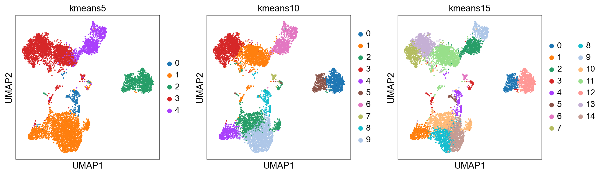
AxisArrays with keys: Scanorama, X_pca, X_pca_harmony, X_tsne, X_tsne_bbknn, X_tsne_harmony, X_tsne_scanorama, X_tsne_uncorr, X_umap, X_umap_bbknn, X_umap_harmony, X_umap_scanorama, X_umap_uncorr3 Hierarchical clustering
Hierarchical clustering is another generic form of clustering that can be applied also to scRNA-seq data. As K-means, it is typically applied to a reduced dimension representation of the data. Hierarchical clustering returns an entire hierarchy of partitionings (a dendrogram) that can be cut at different levels. Hierarchical clustering is done in these steps:
- Define the distances between samples. The most common are Euclidean distance (a.k.a. straight line between two points) or correlation coefficients.
- Define a measure of distances between clusters, called linkage criteria. It can for example be average distances between clusters. Commonly used methods are
single,complete,average,median,centroidandward. - Define the dendrogram among all samples using Bottom-up or Top-down approach. Bottom-up is where samples start with their own cluster which end up merged pair-by-pair until only one cluster is left. Top-down is where samples start all in the same cluster that end up being split by 2 until each sample has its own cluster.
As you might have realized, correlation is not a method implemented in the dist() function. However, we can create our own distances and transform them to a distance object. We can first compute sample correlations using the cor function.
As you already know, correlation range from -1 to 1, where 1 indicates that two samples are closest, -1 indicates that two samples are the furthest and 0 is somewhat in between. This, however, creates a problem in defining distances because a distance of 0 indicates that two samples are closest, 1 indicates that two samples are the furthest and distance of -1 is not meaningful. We thus need to transform the correlations to a positive scale (a.k.a. adjacency):
\[adj = \frac{1- cor}{2}\]
Once we transformed the correlations to a 0-1 scale, we can simply convert it to a distance object using as.dist() function. The transformation does not need to have a maximum of 1, but it is more intuitive to have it at 1, rather than at any other number.
The function AgglomerativeClustering has the option of running with disntance metrics “euclidean”, “l1”, “l2”, “manhattan”, “cosine”, or “precomputed”. However, with ward linkage only euklidean distances works. Here we will try out euclidean distance and ward linkage calculated in PCA space.
from sklearn.cluster import AgglomerativeClustering

cluster = AgglomerativeClustering(n_clusters=5, linkage='ward')
adata.obs['hclust_5'] = cluster.fit_predict(X_pca).astype(str)

cluster = AgglomerativeClustering(n_clusters=10, linkage='ward')
adata.obs['hclust_10'] = cluster.fit_predict(X_pca).astype(str)

cluster = AgglomerativeClustering(n_clusters=15, linkage='ward')
adata.obs['hclust_15'] = cluster.fit_predict(X_pca).astype(str)

sc.pl.umap(adata, color=['hclust_5', 'hclust_10', 'hclust_15'])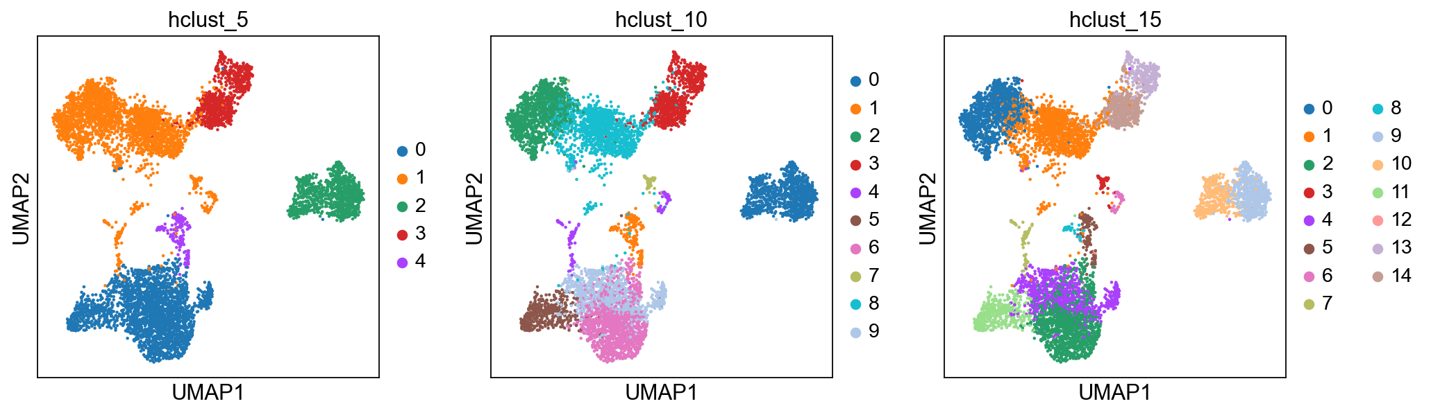
Finally, lets save the clustered data for further analysis.
adata.write_h5ad('./data/covid/results/scanpy_covid_qc_dr_int_cl.h5ad')4 Distribution of clusters
Now, we can select one of our clustering methods and compare the proportion of samples across the clusters.
Select the “leiden_0.6” and plot proportion of samples per cluster and also proportion covid vs ctrl.
Plot proportion of cells from each condition per cluster.
tmp = pd.crosstab(adata.obs['leiden_0.6'],adata.obs['type'], normalize='index')
tmp.plot.bar(stacked=True).legend(bbox_to_anchor=(1.4, 1), loc='upper right')

tmp = pd.crosstab(adata.obs['leiden_0.6'],adata.obs['sample'], normalize='index')
tmp.plot.bar(stacked=True).legend(bbox_to_anchor=(1.4, 1),loc='upper right')
<matplotlib.legend.Legend at 0x7ffe837c8280>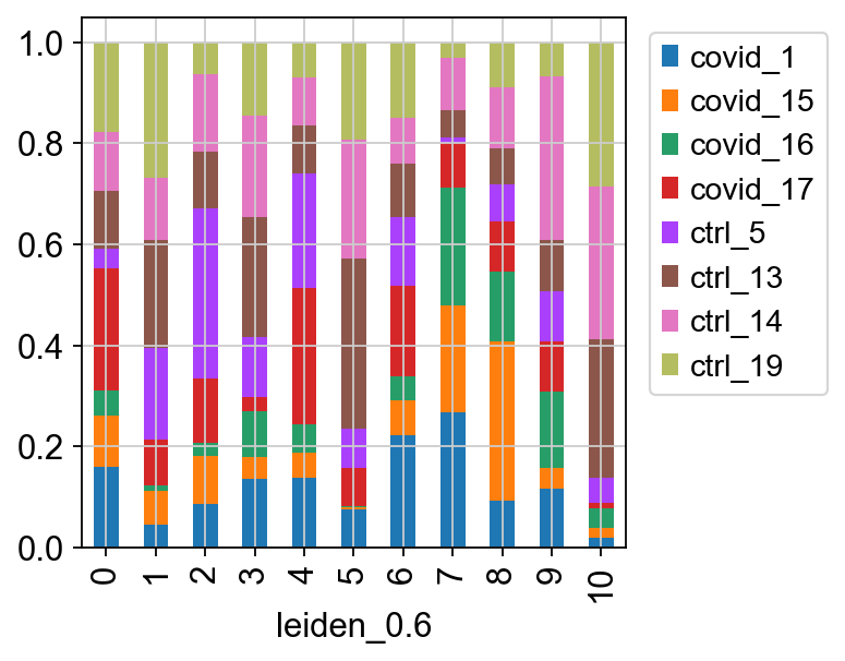
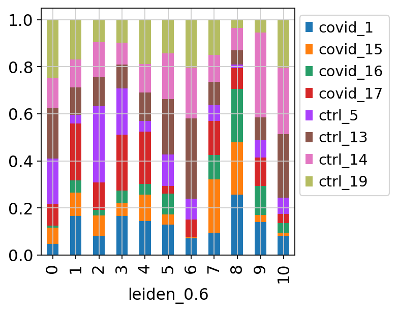
In this case we have quite good representation of each sample in each cluster. But there are clearly some biases with more cells from one sample in some clusters and also more covid cells in some of the clusters.
We can also plot it in the other direction, the proportion of each cluster per sample.
tmp = pd.crosstab(adata.obs['sample'],adata.obs['leiden_0.6'], normalize='index')
tmp.plot.bar(stacked=True).legend(bbox_to_anchor=(1.4, 1), loc='upper right')
<matplotlib.legend.Legend at 0x7ffe8a94e290>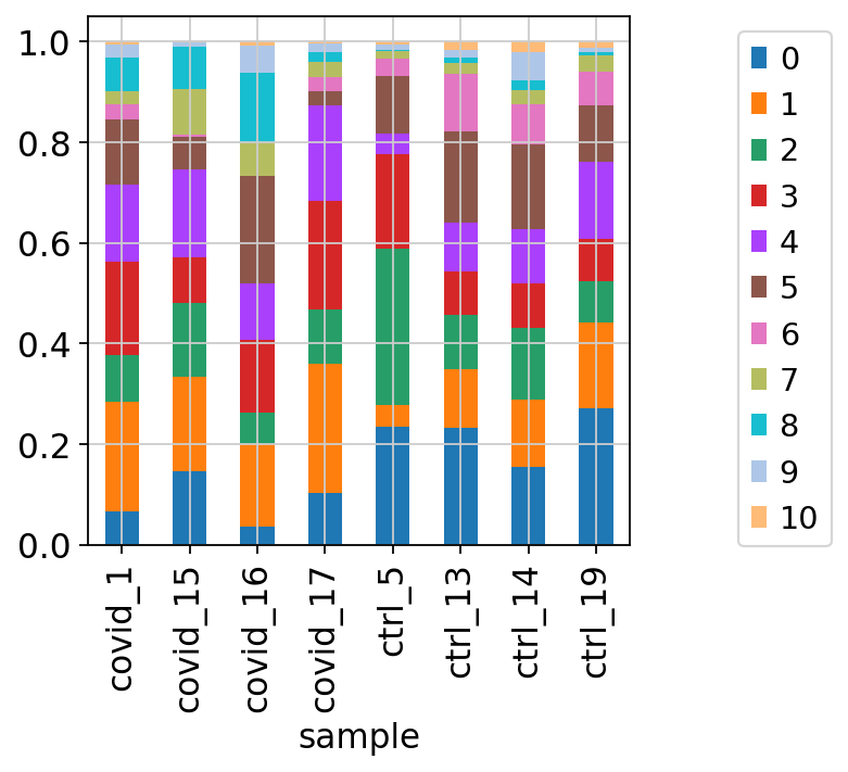
Discuss
By now you should know how to plot different features onto your data. Take the QC metrics that were calculated in the first exercise, that should be stored in your data object, and plot it as violin plots per cluster using the clustering method of your choice. For example, plot number of UMIS, detected genes, percent mitochondrial reads. Then, check carefully if there is any bias in how your data is separated by quality metrics. Could it be explained biologically, or could there be a technical bias there?
sc.pl.violin(adata, ['n_genes_by_counts', 'total_counts', 'pct_counts_mt'], jitter=0.4, groupby = 'leiden_0.6', rotation= 45)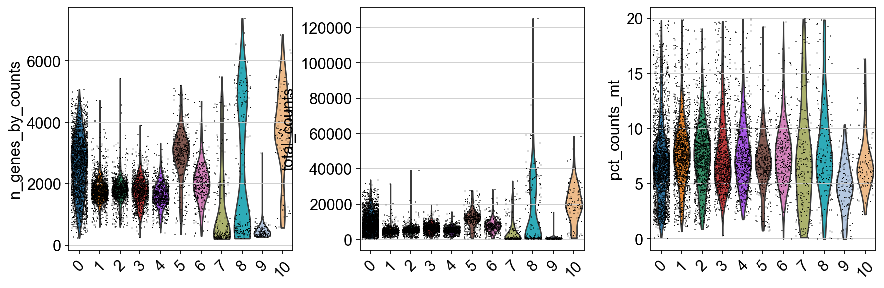
Some clusters that are clearly defined by higher number of genes and counts. These are either doublets or a larger celltype. And some clusters with low values on these metrics that are either low quality cells or a smaller celltype. You will have to explore these clusters in more detail to judge what you believe them to be.
5 Subclustering of T and NK-cells
It is common that the subtypes of cells within a cluster is not so well separated when you have a heterogeneous dataset. In such a case it could be a good idea to run subclustering of individual celltypes. The main reason for subclustering is that the variable genes and the first principal components in the full analysis are mainly driven by differences between celltypes, while with subclustering we may detect smaller differences between subtypes within celltypes.
So first, lets find out where our T-cell and NK-cell clusters are. We know that T-cells express CD3E, and the main subtypes are CD4 and CD8, while NK-cells express GNLY.
# check with the lowest resolution
fig, axs = plt.subplots(2, 3, figsize=(10,8),constrained_layout=True)
sc.pl.umap(adata, color="leiden_0.4", ax=axs[0,0], show=False, legend_loc = "on data")
sc.pl.umap(adata, color="CD3E", ax=axs[0,1], show=False)
sc.pl.umap(adata, color="CD4", ax=axs[0,2], show=False)
sc.pl.umap(adata, color="CD8A", ax=axs[1,0], show=False)
sc.pl.umap(adata, color="GNLY", ax=axs[1,1], show=False)
<Axes: title={'center': 'GNLY'}, xlabel='UMAP1', ylabel='UMAP2'>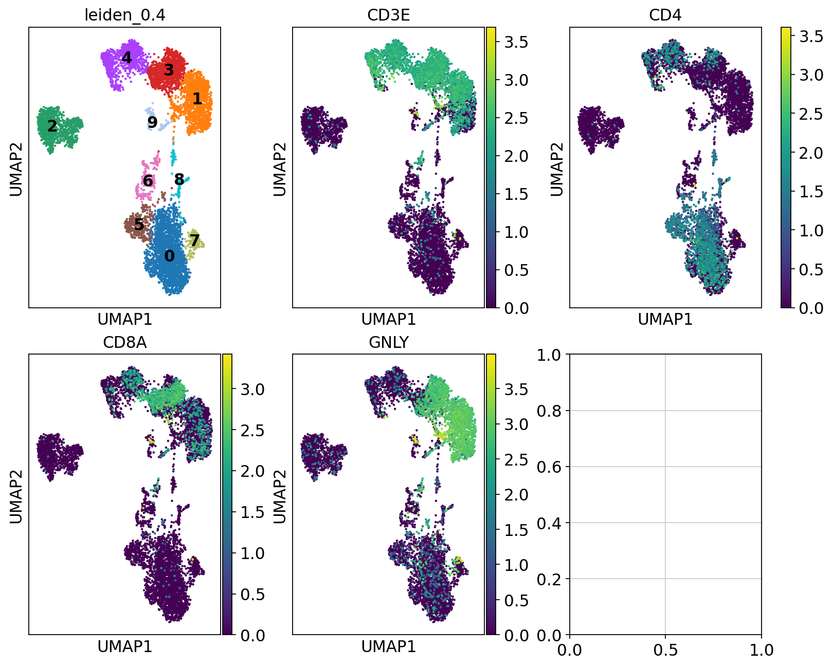
We can clearly see what clusters are T-cell clusters, so lets subset the data for those cells
tcells = adata[adata.obs["leiden_0.4"].isin(['1','3','4']),:]
tcells.obs["sample"].value_counts()
ctrl_5 694
ctrl_13 613
ctrl_19 550
ctrl_14 492
covid_17 278
covid_1 261
covid_15 237
covid_16 122
Name: sample, dtype: int64Ideally we should rerun all steps of integration with that subset of cells instead of just taking the joint embedding. If you have too few cells per sample in the celltype that you want to cluster it may not be possible. We will start with selecting a new set of genes that better reflecs the variability within this celltype
sc.pp.highly_variable_genes(tcells, min_mean=0.0125, max_mean=3, min_disp=0.5)


print("Full data:" , sum(adata.var.highly_variable ))
print("Tcells:" , sum(tcells.var.highly_variable))
print("Intersection:" , sum(tcells.var.highly_variable & adata.var.highly_variable))
extracting highly variable genes
finished (0:00:01)
--> added
'highly_variable', boolean vector (adata.var)
'means', float vector (adata.var)
'dispersions', float vector (adata.var)
'dispersions_norm', float vector (adata.var)
Full data: 2144
Tcells: 2964
Intersection: 928We clearly have a very different geneset now, so hopefully it should better capture the variability within T-cells.
Now we have to run the full pipeline with scaling, pca, integration and clustering on this subset of cells, using the new set of variable genes
import scanpy.external as sce
import harmonypy as hm

tcells.raw = tcells
tcells = tcells[:, tcells.var.highly_variable]
sc.pp.regress_out(tcells, ['total_counts', 'pct_counts_mt'])
sc.pp.scale(tcells, max_value=10)
sc.tl.pca(tcells, svd_solver='arpack')
sce.pp.harmony_integrate(tcells, 'sample')
sc.pp.neighbors(tcells, n_neighbors=10, n_pcs=30, use_rep='X_pca_harmony')
sc.tl.leiden(tcells, resolution = 0.6, key_added = "tcells_0.6")
sc.tl.umap(tcells)
regressing out ['total_counts', 'pct_counts_mt']
sparse input is densified and may lead to high memory use
finished (0:00:16)
computing PCA
with n_comps=50
finished (0:00:02)
computing neighbors
finished: added to `.uns['neighbors']`
`.obsp['distances']`, distances for each pair of neighbors
`.obsp['connectivities']`, weighted adjacency matrix (0:00:00)
running Leiden clustering
finished: found 10 clusters and added
'tcells_0.6', the cluster labels (adata.obs, categorical) (0:00:00)
computing UMAP
finished: added
'X_umap', UMAP coordinates (adata.obsm)
'umap', UMAP parameters (adata.uns) (0:00:04)fig, axs = plt.subplots(2, 3, figsize=(10,8),constrained_layout=True)
sc.pl.umap(tcells, color="sample", title="Tcell umap", ax=axs[0,0], show=False)
sc.pl.embedding(tcells, 'X_umap_harmony', color="sample", title="Full umap", ax=axs[1,0], show=False)
sc.pl.umap(tcells, color="leiden_0.6", title="Tcell umap, full clust", ax=axs[0,1], show=False)
sc.pl.embedding(tcells, 'X_umap_harmony', color="leiden_0.6", title="Full umap, full clust", ax=axs[1,1], show=False)
sc.pl.umap(tcells, color="tcells_0.6", title="Tcell umap, tcell clust", ax=axs[0,2], show=False)
sc.pl.embedding(tcells, 'X_umap_harmony', color="tcells_0.6", title="Full umap, tcell clust", ax=axs[1,2], show=False)<Axes: title={'center': 'Full umap, tcell clust'}, xlabel='X_umap_harmony1', ylabel='X_umap_harmony2'>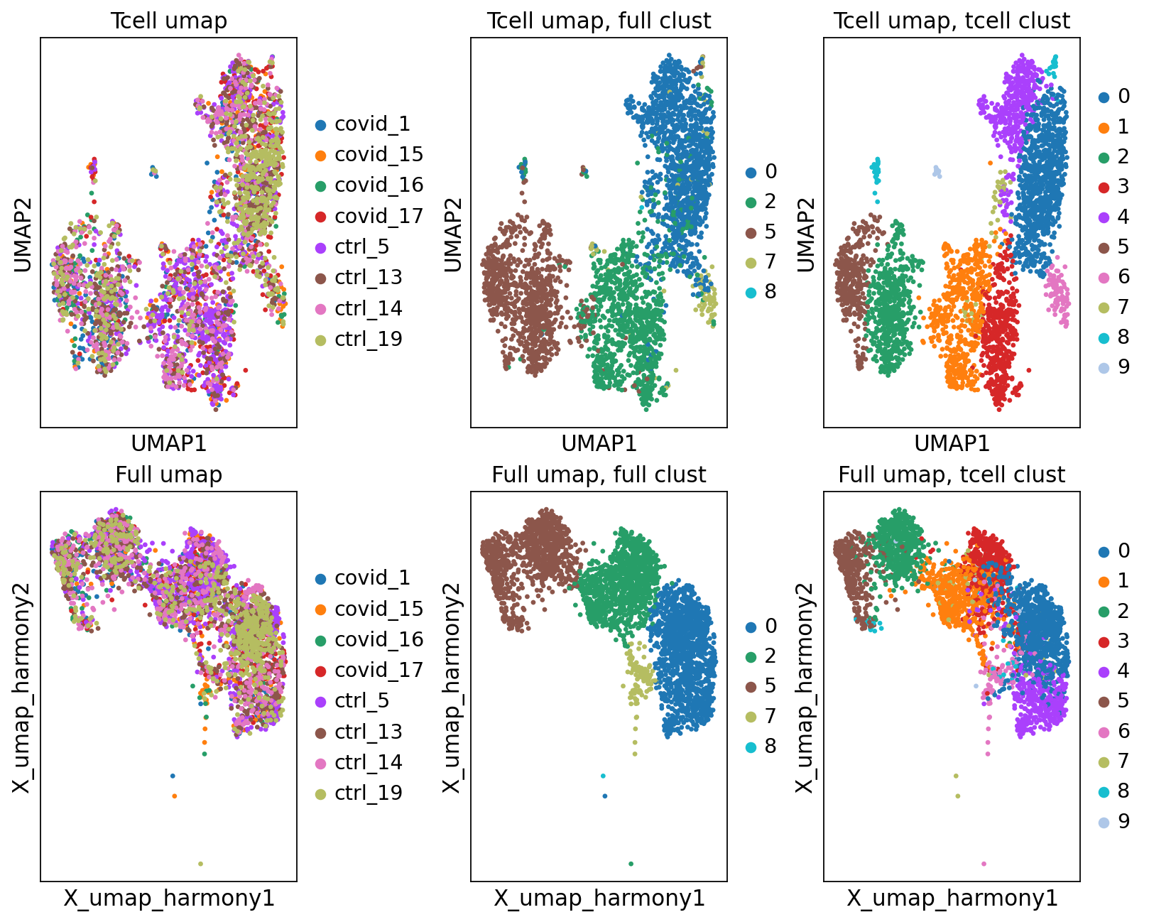
As you can see, we do have some new clusters that did not stand out before. But in general the separation looks very similar.
We can plot the subtype genes again. If you try plotting the genes with use_raw=False you will notice that some of the genes are not in the adata.X matrix. Since they are no longer included in the variable genes. So now we have to plot with use_raw=True.
fig, axs = plt.subplots(2, 2, figsize=(10,8),constrained_layout=True)
sc.pl.umap(tcells, color="CD3E", ax=axs[0,0], show=False, use_raw=True)
sc.pl.umap(tcells, color="CD4", ax=axs[0,1], show=False, use_raw=True)
sc.pl.umap(tcells, color="CD8A", ax=axs[1,0], show=False, use_raw=True)
sc.pl.umap(tcells, color="GNLY", ax=axs[1,1], show=False, use_raw=True)
<Axes: title={'center': 'GNLY'}, xlabel='UMAP1', ylabel='UMAP2'>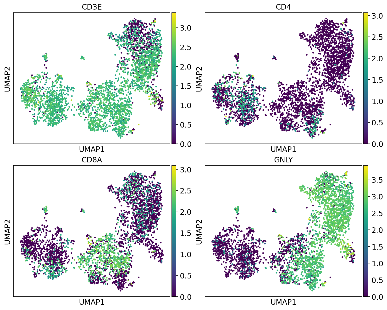
Discuss
Have a look at the T-cells in the umaps with all cells or only T/NK cells. What are the main differences? Do you think it improved with subclustering? Also, there are some cells in these clusters that fall far away from the rest in the UMAPs, why do you think that is?
6 Session info
Click here
sc.logging.print_versions()-----
anndata 0.10.8
scanpy 1.10.3
-----
PIL 11.1.0
asttokens NA
cffi 1.17.1
colorama 0.4.6
comm 0.2.2
cycler 0.12.1
cython_runtime NA
dateutil 2.9.0.post0
debugpy 1.8.12
decorator 5.1.1
exceptiongroup 1.2.2
executing 2.1.0
h5py 3.12.1
harmonypy 0.0.10
igraph 0.11.6
ipykernel 6.29.5
jedi 0.19.2
joblib 1.4.2
kiwisolver 1.4.7
legacy_api_wrap NA
leidenalg 0.10.2
llvmlite 0.43.0
matplotlib 3.9.2
matplotlib_inline 0.1.7
mpl_toolkits NA
natsort 8.4.0
numba 0.60.0
numpy 1.26.4
packaging 24.2
pandas 1.5.3
parso 0.8.4
patsy 1.0.1
pickleshare 0.7.5
platformdirs 4.3.6
prompt_toolkit 3.0.50
psutil 6.1.1
pure_eval 0.2.3
pycparser 2.22
pydev_ipython NA
pydevconsole NA
pydevd 3.2.3
pydevd_file_utils NA
pydevd_plugins NA
pydevd_tracing NA
pygments 2.19.1
pynndescent 0.5.13
pyparsing 3.2.1
pytz 2024.2
scipy 1.14.1
seaborn 0.13.2
session_info 1.0.0
six 1.17.0
sklearn 1.6.1
sparse 0.15.5
stack_data 0.6.3
statsmodels 0.14.4
texttable 1.7.0
threadpoolctl 3.5.0
torch 2.5.1.post207
torchgen NA
tornado 6.4.2
tqdm 4.67.1
traitlets 5.14.3
typing_extensions NA
umap 0.5.7
wcwidth 0.2.13
yaml 6.0.2
zmq 26.2.0
zoneinfo NA
-----
IPython 8.31.0
jupyter_client 8.6.3
jupyter_core 5.7.2
-----
Python 3.10.16 | packaged by conda-forge | (main, Dec 5 2024, 14:16:10) [GCC 13.3.0]
Linux-6.10.14-linuxkit-x86_64-with-glibc2.35
-----
Session information updated at 2025-02-27 15:17