import numpy as np
import pandas as pd
import scanpy as sc
import matplotlib.pyplot as plt
import warnings
import os
import subprocess

warnings.simplefilter(action='ignore', category=Warning)

# verbosity: errors (0), warnings (1), info (2), hints (3)
sc.settings.verbosity = 3

sc.settings.set_figure_params(dpi=80)
%matplotlib inline
Note
Code chunks run Python commands unless it starts with %%bash, in which case, those chunks run shell commands.
In this tutorial we will look at different ways of integrating multiple single cell RNA-seq datasets. We will explore a few different methods to correct for batch effects across datasets. Seurat uses the data integration method presented in Comprehensive Integration of Single Cell Data, while Scran and Scanpy use a mutual Nearest neighbour method (MNN). Below you can find a list of some methods for single data integration:
| Markdown | Language | Library | Ref |
|---|---|---|---|
| CCA | R | Seurat | Cell |
| MNN | R/Python | Scater/Scanpy | Nat. Biotech. |
| Conos | R | conos | Nat. Methods |
| Scanorama | Python | scanorama | Nat. Biotech. |
1 Data preparation
Let’s first load necessary libraries and the data saved in the previous lab.
Create individual adata objects per batch.
# download pre-computed data if missing or long compute
fetch_data = True

# url for source and intermediate data
path_data = "https://nextcloud.dc.scilifelab.se/public.php/webdav"
curl_upass = "zbC5fr2LbEZ9rSE:scRNAseq2025"


path_results = "data/covid/results"
if not os.path.exists(path_results):
    os.makedirs(path_results, exist_ok=True)

path_file = "data/covid/results/scanpy_covid_qc_dr.h5ad"
if fetch_data and not os.path.exists(path_file):
    file_url = os.path.join(path_data, "covid/results_scanpy/scanpy_covid_qc_dr.h5ad")
    subprocess.call(["curl", "-u", curl_upass, "-o", path_file, file_url ])

adata = sc.read_h5ad(path_file)
adata
AnnData object with n_obs × n_vars = 7332 × 2656
obs: 'type', 'sample', 'batch', 'n_genes_by_counts', 'total_counts', 'total_counts_mt', 'pct_counts_mt', 'total_counts_ribo', 'pct_counts_ribo', 'total_counts_hb', 'pct_counts_hb', 'percent_mt2', 'n_counts', 'n_genes', 'percent_chrY', 'XIST-counts', 'S_score', 'G2M_score', 'phase', 'doublet_scores', 'predicted_doublets', 'doublet_info'
var: 'gene_ids', 'feature_types', 'genome', 'mt', 'ribo', 'hb', 'n_cells_by_counts', 'mean_counts', 'pct_dropout_by_counts', 'total_counts', 'n_cells', 'highly_variable', 'means', 'dispersions', 'dispersions_norm', 'mean', 'std'
uns: 'doublet_info_colors', 'hvg', 'log1p', 'neighbors', 'pca', 'phase_colors', 'sample_colors', 'tsne', 'umap'
obsm: 'X_pca', 'X_tsne', 'X_umap'
varm: 'PCs'
obsp: 'connectivities', 'distances'print(adata.X.shape)(7332, 2656)As the stored AnnData object contains scaled data based on variable genes, we need to make a new object with the logtransformed normalized counts. The new variable gene selection should not be performed on the scaled data matrix.
adata2 = adata.raw.to_adata()

# in some versions of Anndata there is an issue with information on the logtransformation in the slot log1p.base so we set it to None to not get errors.
adata2.uns['log1p']['base']=None

# check that the matrix looks like normalized counts
print(adata2.X[1:10,1:10])
<Compressed Sparse Row sparse matrix of dtype 'float64'
with 2 stored elements and shape (9, 9)>
Coords Values
(0, 3) 1.479703103222477
(7, 6) 1.63974082378425322 Detect variable genes
Variable genes can be detected across the full dataset, but then we run the risk of getting many batch-specific genes that will drive a lot of the variation. Or we can select variable genes from each batch separately to get only celltype variation. In the dimensionality reduction exercise, we already selected variable genes, so they are already stored in adata.var.highly_variable.
var_genes_all = adata.var.highly_variable

print("Highly variable genes: %d"%sum(var_genes_all))
Highly variable genes: 2656Detect variable genes in each dataset separately using the batch_key parameter.
sc.pp.highly_variable_genes(adata2, min_mean=0.0125, max_mean=3, min_disp=0.5, batch_key = 'sample')

print("Highly variable genes intersection: %d"%sum(adata2.var.highly_variable_intersection))

print("Number of batches where gene is variable:")
print(adata2.var.highly_variable_nbatches.value_counts())

var_genes_batch = adata2.var.highly_variable_nbatches > 0
extracting highly variable genes
finished (0:00:03)
--> added
'highly_variable', boolean vector (adata.var)
'means', float vector (adata.var)
'dispersions', float vector (adata.var)
'dispersions_norm', float vector (adata.var)
Highly variable genes intersection: 83
Number of batches where gene is variable:
0 6760
1 5164
2 3560
3 2050
4 1003
5 487
6 228
7 133
8 83
Name: highly_variable_nbatches, dtype: int64Compare overlap of variable genes with batches or with all data.
print("Any batch var genes: %d"%sum(var_genes_batch))
print("All data var genes: %d"%sum(var_genes_all))
print("Overlap: %d"%sum(var_genes_batch & var_genes_all))
print("Variable genes in all batches: %d"%sum(adata2.var.highly_variable_nbatches == 6))
print("Overlap batch instersection and all: %d"%sum(var_genes_all & adata2.var.highly_variable_intersection))
Any batch var genes: 12708
All data var genes: 2656
Overlap: 2654
Variable genes in all batches: 228
Overlap batch instersection and all: 83
Discuss
Did you understand the difference between running variable gene selection per dataset and combining them vs running it on all samples together. Can you think of any situation where it would be best to run it on all samples and a situation where it should be done by batch?
Select all genes that are variable in at least 2 datasets and use for remaining analysis.
var_select = adata2.var.highly_variable_nbatches > 2
var_genes = var_select.index[var_select]
len(var_genes)39843 BBKNN
First, we will run BBKNN that is implemented in scanpy.
import bbknn
bbknn.bbknn(adata2,batch_key='sample')

# Before calculating a new umap and tsne, we want to store the old one.
adata2.obsm['X_umap_uncorr'] = adata2.obsm['X_umap']
adata2.obsm['X_tsne_uncorr'] = adata2.obsm['X_tsne']


# then run umap on the integrated space
sc.tl.umap(adata2)
sc.tl.tsne(adata2)
computing batch balanced neighbors
finished: added to `.uns['neighbors']`
`.obsp['distances']`, distances for each pair of neighbors
`.obsp['connectivities']`, weighted adjacency matrix (0:00:02)
computing UMAP
finished: added
'X_umap', UMAP coordinates (adata.obsm)
'umap', UMAP parameters (adata.uns) (0:00:13)
computing tSNE
using 'X_pca' with n_pcs = 50
using sklearn.manifold.TSNE
finished: added
'X_tsne', tSNE coordinates (adata.obsm)
'tsne', tSNE parameters (adata.uns) (0:00:48)We can now plot the unintegrated and the integrated space reduced dimensions.
fig, axs = plt.subplots(2, 2, figsize=(10,8),constrained_layout=True)
sc.pl.tsne(adata2, color="sample", title="BBKNN Corrected tsne", ax=axs[0,0], show=False)
sc.pl.tsne(adata, color="sample", title="Uncorrected tsne", ax=axs[0,1], show=False)
sc.pl.umap(adata2, color="sample", title="BBKNN Corrected umap", ax=axs[1,0], show=False)
sc.pl.umap(adata, color="sample", title="Uncorrected umap", ax=axs[1,1], show=False)
<Axes: title={'center': 'Uncorrected umap'}, xlabel='UMAP1', ylabel='UMAP2'>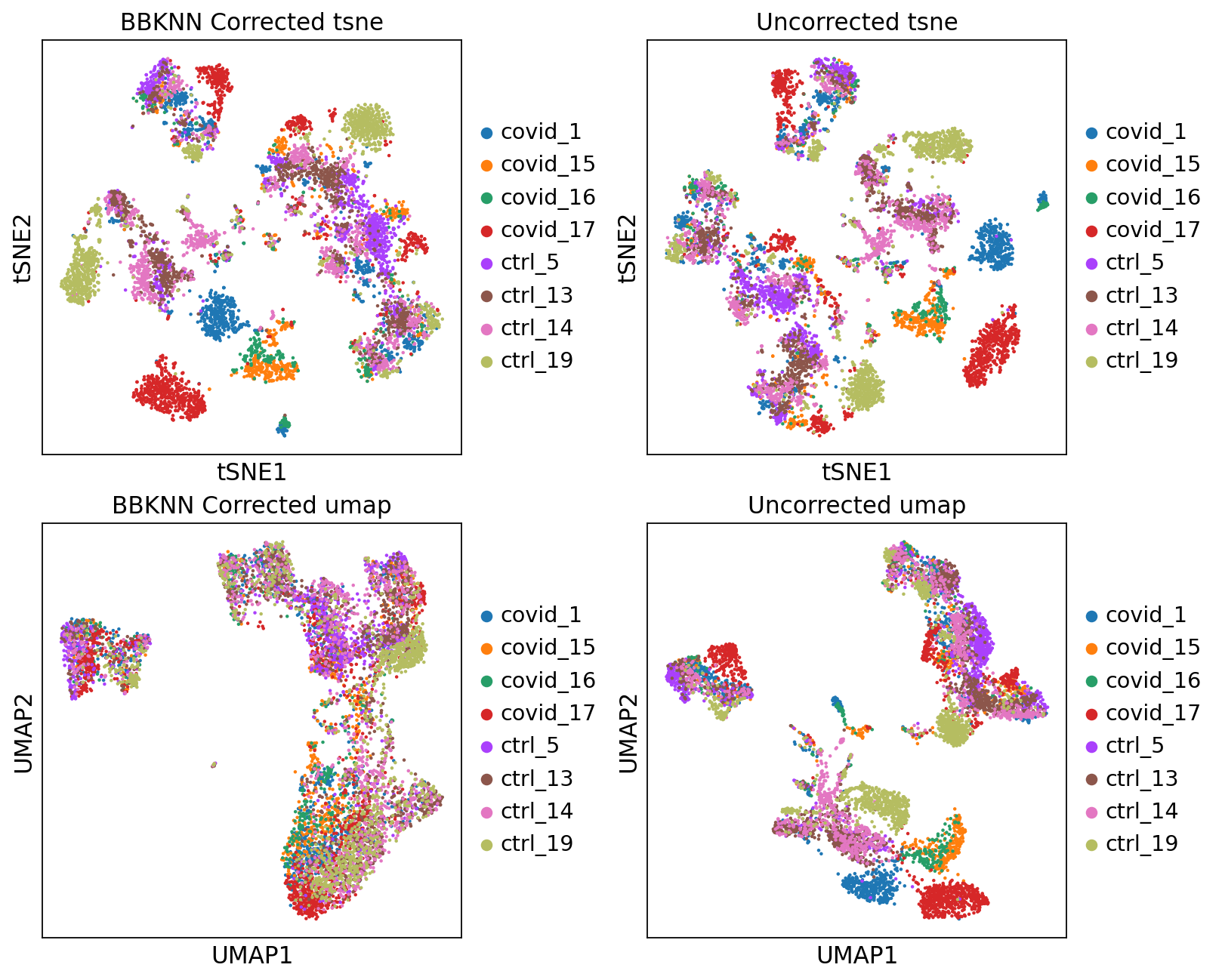
Let’s save the integrated data for further analysis.
# Before calculating a new umap and tsne, we want to store the old one.
adata2.obsm['X_umap_bbknn'] = adata2.obsm['X_umap']
adata2.obsm['X_tsne_bbknn'] = adata2.obsm['X_tsne']

save_file = './data/covid/results/scanpy_covid_qc_dr_bbknn.h5ad'
adata2.write_h5ad(save_file)
4 Harmony
An alternative method for integration is Harmony, for more details on the method, please se their paper Nat. Methods. This method runs the integration on a dimensionality reduction, in most applications the PCA.
import scanpy.external as sce
import harmonypy as hm

sce.pp.harmony_integrate(adata2, 'sample')

# Then we calculate a new umap and tsne.
sc.pp.neighbors(adata2, n_neighbors=10, n_pcs=30, use_rep='X_pca_harmony')
sc.tl.umap(adata2)
sc.tl.tsne(adata2, use_rep='X_pca_harmony')
sc.tl.leiden(adata2, resolution=0.5)
computing neighbors
finished: added to `.uns['neighbors']`
`.obsp['distances']`, distances for each pair of neighbors
`.obsp['connectivities']`, weighted adjacency matrix (0:00:01)
computing UMAP
finished: added
'X_umap', UMAP coordinates (adata.obsm)
'umap', UMAP parameters (adata.uns) (0:00:09)
computing tSNE
using sklearn.manifold.TSNE
finished: added
'X_tsne', tSNE coordinates (adata.obsm)
'tsne', tSNE parameters (adata.uns) (0:00:49)
running Leiden clustering
finished: found 11 clusters and added
'leiden', the cluster labels (adata.obs, categorical) (0:00:00)fig, axs = plt.subplots(2, 2, figsize=(10,8),constrained_layout=True)
sc.pl.embedding(adata2, 'X_tsne_bbknn', color="sample", title="BBKNN tsne", ax=axs[0,0], show=False)
sc.pl.tsne(adata2, color="sample", title="Harmony tsne", ax=axs[0,1], show=False)
sc.pl.embedding(adata2, 'X_umap_bbknn', color="sample", title="BBKNN umap", ax=axs[1,0], show=False)
sc.pl.umap(adata2, color="sample", title="Harmony umap", ax=axs[1,1], show=False)<Axes: title={'center': 'Harmony umap'}, xlabel='UMAP1', ylabel='UMAP2'>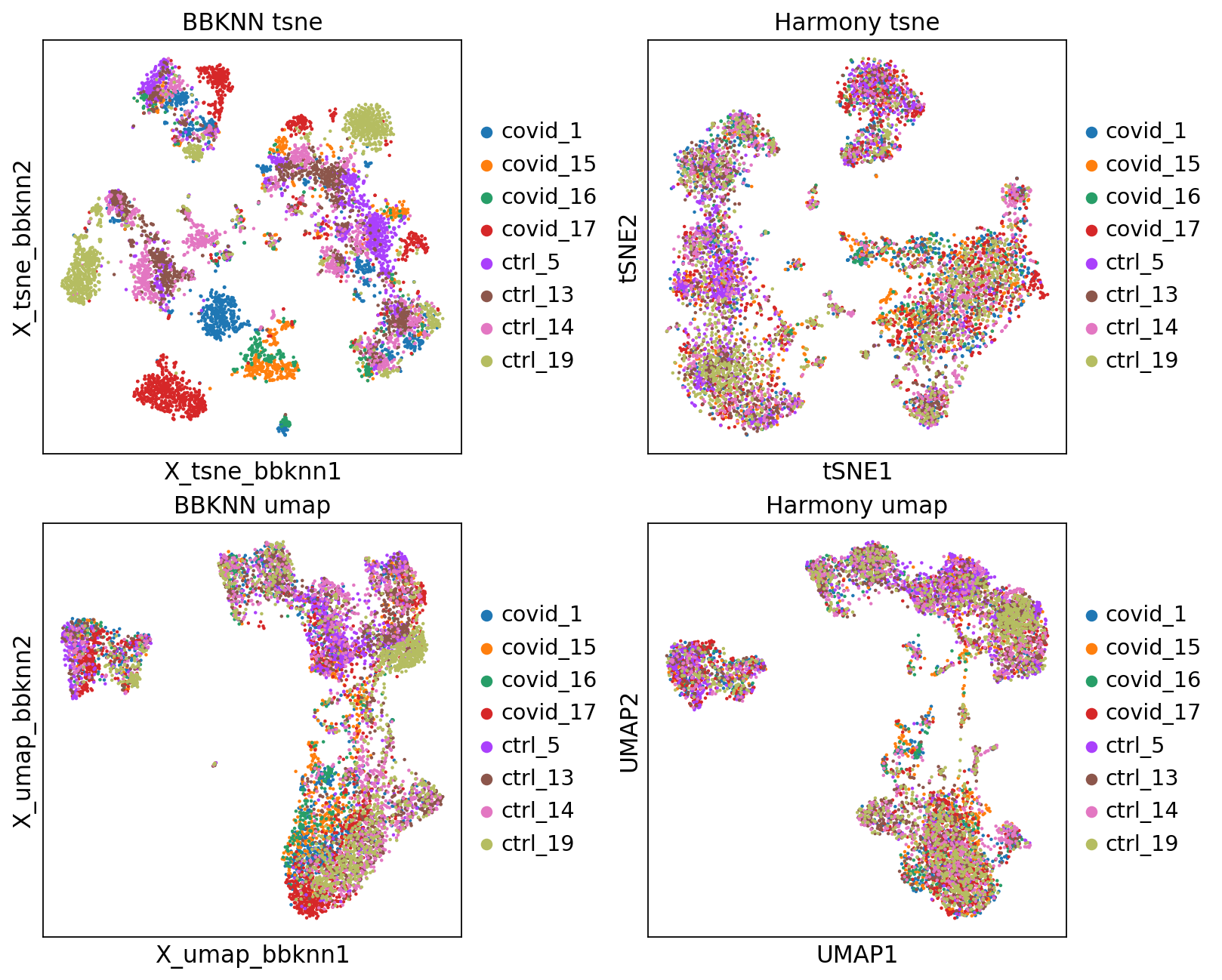
Let’s save the integrated data for further analysis.
# Store this umap and tsne with a new name.
adata2.obsm['X_umap_harmony'] = adata2.obsm['X_umap']
adata2.obsm['X_tsne_harmony'] = adata2.obsm['X_tsne']

#save to file
save_file = './data/covid/results/scanpy_covid_qc_dr_harmony.h5ad'
adata2.write_h5ad(save_file)
5 Combat
Batch correction can also be performed with combat. Note that ComBat batch correction requires a dense matrix format as input (which is already the case in this example).
# create a new object with lognormalized counts
adata_combat = sc.AnnData(X=adata.raw.X, var=adata.raw.var, obs = adata.obs)

# first store the raw data
adata_combat.raw = adata_combat

# run combat
sc.pp.combat(adata_combat, key='sample')
Standardizing Data across genes.
Found 8 batches
Found 0 numerical variables:
Found 34 genes with zero variance.
Fitting L/S model and finding priors
Finding parametric adjustments
Adjusting data
Then we run the regular steps of dimensionality reduction on the combat corrected data. Variable gene selection, pca and umap with combat data.
sc.pp.highly_variable_genes(adata_combat)
print("Highly variable genes: %d"%sum(adata_combat.var.highly_variable))
sc.pl.highly_variable_genes(adata_combat)

sc.pp.pca(adata_combat, n_comps=30, use_highly_variable=True, svd_solver='arpack')

sc.pp.neighbors(adata_combat)

sc.tl.umap(adata_combat)
sc.tl.tsne(adata_combat)
extracting highly variable genes
finished (0:00:01)
--> added
'highly_variable', boolean vector (adata.var)
'means', float vector (adata.var)
'dispersions', float vector (adata.var)
'dispersions_norm', float vector (adata.var)
Highly variable genes: 3271
computing PCA
with n_comps=30
finished (0:00:01)
computing neighbors
using 'X_pca' with n_pcs = 30
finished: added to `.uns['neighbors']`
`.obsp['distances']`, distances for each pair of neighbors
`.obsp['connectivities']`, weighted adjacency matrix (0:00:00)
computing UMAP
finished: added
'X_umap', UMAP coordinates (adata.obsm)
'umap', UMAP parameters (adata.uns) (0:00:10)
computing tSNE
using 'X_pca' with n_pcs = 30
using sklearn.manifold.TSNE
finished: added
'X_tsne', tSNE coordinates (adata.obsm)
'tsne', tSNE parameters (adata.uns) (0:00:45)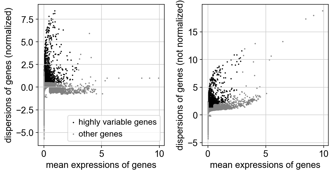
# compare var_genes
var_genes_combat = adata_combat.var.highly_variable
print("With all data %d"%sum(var_genes_all))
print("With combat %d"%sum(var_genes_combat))
print("Overlap %d"%sum(var_genes_all & var_genes_combat))

print("With 2 batches %d"%sum(var_select))
print("Overlap %d"%sum(var_genes_combat & var_select))
With all data 2656
With combat 3271
Overlap 1466
With 2 batches 3984
Overlap 1815We can now plot the unintegrated and the integrated space reduced dimensions.
fig, axs = plt.subplots(2, 2, figsize=(10,8),constrained_layout=True)
sc.pl.tsne(adata2, color="sample", title="Harmony tsne", ax=axs[0,0], show=False)
sc.pl.tsne(adata_combat, color="sample", title="Combat tsne", ax=axs[0,1], show=False)
sc.pl.umap(adata2, color="sample", title="Harmony umap", ax=axs[1,0], show=False)
sc.pl.umap(adata_combat, color="sample", title="Combat umap", ax=axs[1,1], show=False)
<Axes: title={'center': 'Combat umap'}, xlabel='UMAP1', ylabel='UMAP2'>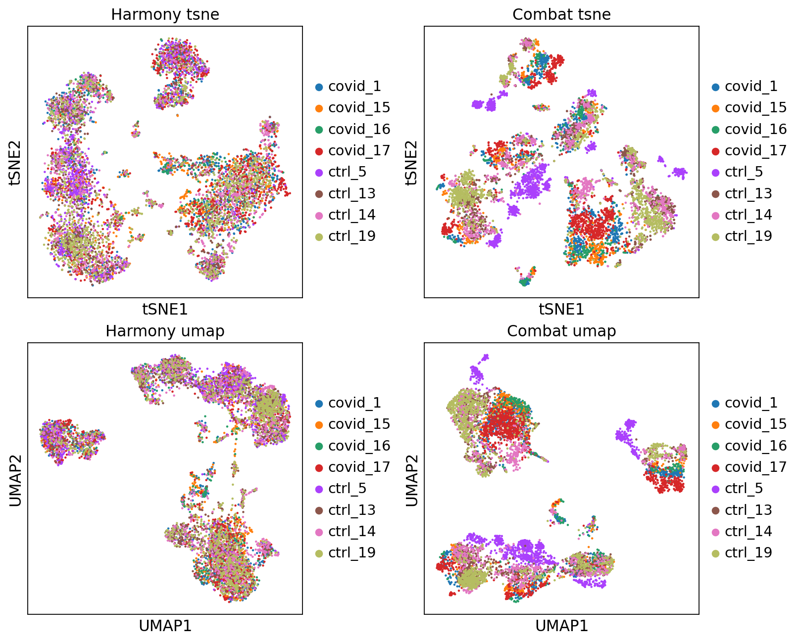
Let’s save the integrated data for further analysis.
#save to file
save_file = './data/covid/results/scanpy_covid_qc_dr_combat.h5ad'
adata_combat.write_h5ad(save_file)
6 Scanorama
Try out Scanorama for data integration as well. First we need to create individual AnnData objects from each of the datasets.
# split per batch into new objects.
batches = adata2.obs['sample'].cat.categories.tolist()
alldata = {}
for batch in batches:
    alldata[batch] = adata2[adata2.obs['sample'] == batch,]

alldata
{'covid_1': View of AnnData object with n_obs × n_vars = 888 × 19468
obs: 'type', 'sample', 'batch', 'n_genes_by_counts', 'total_counts', 'total_counts_mt', 'pct_counts_mt', 'total_counts_ribo', 'pct_counts_ribo', 'total_counts_hb', 'pct_counts_hb', 'percent_mt2', 'n_counts', 'n_genes', 'percent_chrY', 'XIST-counts', 'S_score', 'G2M_score', 'phase', 'doublet_scores', 'predicted_doublets', 'doublet_info', 'leiden'
var: 'gene_ids', 'feature_types', 'genome', 'mt', 'ribo', 'hb', 'n_cells_by_counts', 'mean_counts', 'pct_dropout_by_counts', 'total_counts', 'n_cells', 'highly_variable', 'means', 'dispersions', 'dispersions_norm', 'highly_variable_nbatches', 'highly_variable_intersection'
uns: 'doublet_info_colors', 'hvg', 'log1p', 'neighbors', 'pca', 'phase_colors', 'sample_colors', 'tsne', 'umap', 'leiden'
obsm: 'X_pca', 'X_tsne', 'X_umap', 'X_umap_uncorr', 'X_tsne_uncorr', 'X_umap_bbknn', 'X_tsne_bbknn', 'X_pca_harmony', 'X_umap_harmony', 'X_tsne_harmony'
obsp: 'connectivities', 'distances',
'covid_15': View of AnnData object with n_obs × n_vars = 599 × 19468
obs: 'type', 'sample', 'batch', 'n_genes_by_counts', 'total_counts', 'total_counts_mt', 'pct_counts_mt', 'total_counts_ribo', 'pct_counts_ribo', 'total_counts_hb', 'pct_counts_hb', 'percent_mt2', 'n_counts', 'n_genes', 'percent_chrY', 'XIST-counts', 'S_score', 'G2M_score', 'phase', 'doublet_scores', 'predicted_doublets', 'doublet_info', 'leiden'
var: 'gene_ids', 'feature_types', 'genome', 'mt', 'ribo', 'hb', 'n_cells_by_counts', 'mean_counts', 'pct_dropout_by_counts', 'total_counts', 'n_cells', 'highly_variable', 'means', 'dispersions', 'dispersions_norm', 'highly_variable_nbatches', 'highly_variable_intersection'
uns: 'doublet_info_colors', 'hvg', 'log1p', 'neighbors', 'pca', 'phase_colors', 'sample_colors', 'tsne', 'umap', 'leiden'
obsm: 'X_pca', 'X_tsne', 'X_umap', 'X_umap_uncorr', 'X_tsne_uncorr', 'X_umap_bbknn', 'X_tsne_bbknn', 'X_pca_harmony', 'X_umap_harmony', 'X_tsne_harmony'
obsp: 'connectivities', 'distances',
'covid_16': View of AnnData object with n_obs × n_vars = 371 × 19468
obs: 'type', 'sample', 'batch', 'n_genes_by_counts', 'total_counts', 'total_counts_mt', 'pct_counts_mt', 'total_counts_ribo', 'pct_counts_ribo', 'total_counts_hb', 'pct_counts_hb', 'percent_mt2', 'n_counts', 'n_genes', 'percent_chrY', 'XIST-counts', 'S_score', 'G2M_score', 'phase', 'doublet_scores', 'predicted_doublets', 'doublet_info', 'leiden'
var: 'gene_ids', 'feature_types', 'genome', 'mt', 'ribo', 'hb', 'n_cells_by_counts', 'mean_counts', 'pct_dropout_by_counts', 'total_counts', 'n_cells', 'highly_variable', 'means', 'dispersions', 'dispersions_norm', 'highly_variable_nbatches', 'highly_variable_intersection'
uns: 'doublet_info_colors', 'hvg', 'log1p', 'neighbors', 'pca', 'phase_colors', 'sample_colors', 'tsne', 'umap', 'leiden'
obsm: 'X_pca', 'X_tsne', 'X_umap', 'X_umap_uncorr', 'X_tsne_uncorr', 'X_umap_bbknn', 'X_tsne_bbknn', 'X_pca_harmony', 'X_umap_harmony', 'X_tsne_harmony'
obsp: 'connectivities', 'distances',
'covid_17': View of AnnData object with n_obs × n_vars = 1090 × 19468
obs: 'type', 'sample', 'batch', 'n_genes_by_counts', 'total_counts', 'total_counts_mt', 'pct_counts_mt', 'total_counts_ribo', 'pct_counts_ribo', 'total_counts_hb', 'pct_counts_hb', 'percent_mt2', 'n_counts', 'n_genes', 'percent_chrY', 'XIST-counts', 'S_score', 'G2M_score', 'phase', 'doublet_scores', 'predicted_doublets', 'doublet_info', 'leiden'
var: 'gene_ids', 'feature_types', 'genome', 'mt', 'ribo', 'hb', 'n_cells_by_counts', 'mean_counts', 'pct_dropout_by_counts', 'total_counts', 'n_cells', 'highly_variable', 'means', 'dispersions', 'dispersions_norm', 'highly_variable_nbatches', 'highly_variable_intersection'
uns: 'doublet_info_colors', 'hvg', 'log1p', 'neighbors', 'pca', 'phase_colors', 'sample_colors', 'tsne', 'umap', 'leiden'
obsm: 'X_pca', 'X_tsne', 'X_umap', 'X_umap_uncorr', 'X_tsne_uncorr', 'X_umap_bbknn', 'X_tsne_bbknn', 'X_pca_harmony', 'X_umap_harmony', 'X_tsne_harmony'
obsp: 'connectivities', 'distances',
'ctrl_5': View of AnnData object with n_obs × n_vars = 1039 × 19468
obs: 'type', 'sample', 'batch', 'n_genes_by_counts', 'total_counts', 'total_counts_mt', 'pct_counts_mt', 'total_counts_ribo', 'pct_counts_ribo', 'total_counts_hb', 'pct_counts_hb', 'percent_mt2', 'n_counts', 'n_genes', 'percent_chrY', 'XIST-counts', 'S_score', 'G2M_score', 'phase', 'doublet_scores', 'predicted_doublets', 'doublet_info', 'leiden'
var: 'gene_ids', 'feature_types', 'genome', 'mt', 'ribo', 'hb', 'n_cells_by_counts', 'mean_counts', 'pct_dropout_by_counts', 'total_counts', 'n_cells', 'highly_variable', 'means', 'dispersions', 'dispersions_norm', 'highly_variable_nbatches', 'highly_variable_intersection'
uns: 'doublet_info_colors', 'hvg', 'log1p', 'neighbors', 'pca', 'phase_colors', 'sample_colors', 'tsne', 'umap', 'leiden'
obsm: 'X_pca', 'X_tsne', 'X_umap', 'X_umap_uncorr', 'X_tsne_uncorr', 'X_umap_bbknn', 'X_tsne_bbknn', 'X_pca_harmony', 'X_umap_harmony', 'X_tsne_harmony'
obsp: 'connectivities', 'distances',
'ctrl_13': View of AnnData object with n_obs × n_vars = 1154 × 19468
obs: 'type', 'sample', 'batch', 'n_genes_by_counts', 'total_counts', 'total_counts_mt', 'pct_counts_mt', 'total_counts_ribo', 'pct_counts_ribo', 'total_counts_hb', 'pct_counts_hb', 'percent_mt2', 'n_counts', 'n_genes', 'percent_chrY', 'XIST-counts', 'S_score', 'G2M_score', 'phase', 'doublet_scores', 'predicted_doublets', 'doublet_info', 'leiden'
var: 'gene_ids', 'feature_types', 'genome', 'mt', 'ribo', 'hb', 'n_cells_by_counts', 'mean_counts', 'pct_dropout_by_counts', 'total_counts', 'n_cells', 'highly_variable', 'means', 'dispersions', 'dispersions_norm', 'highly_variable_nbatches', 'highly_variable_intersection'
uns: 'doublet_info_colors', 'hvg', 'log1p', 'neighbors', 'pca', 'phase_colors', 'sample_colors', 'tsne', 'umap', 'leiden'
obsm: 'X_pca', 'X_tsne', 'X_umap', 'X_umap_uncorr', 'X_tsne_uncorr', 'X_umap_bbknn', 'X_tsne_bbknn', 'X_pca_harmony', 'X_umap_harmony', 'X_tsne_harmony'
obsp: 'connectivities', 'distances',
'ctrl_14': View of AnnData object with n_obs × n_vars = 1039 × 19468
obs: 'type', 'sample', 'batch', 'n_genes_by_counts', 'total_counts', 'total_counts_mt', 'pct_counts_mt', 'total_counts_ribo', 'pct_counts_ribo', 'total_counts_hb', 'pct_counts_hb', 'percent_mt2', 'n_counts', 'n_genes', 'percent_chrY', 'XIST-counts', 'S_score', 'G2M_score', 'phase', 'doublet_scores', 'predicted_doublets', 'doublet_info', 'leiden'
var: 'gene_ids', 'feature_types', 'genome', 'mt', 'ribo', 'hb', 'n_cells_by_counts', 'mean_counts', 'pct_dropout_by_counts', 'total_counts', 'n_cells', 'highly_variable', 'means', 'dispersions', 'dispersions_norm', 'highly_variable_nbatches', 'highly_variable_intersection'
uns: 'doublet_info_colors', 'hvg', 'log1p', 'neighbors', 'pca', 'phase_colors', 'sample_colors', 'tsne', 'umap', 'leiden'
obsm: 'X_pca', 'X_tsne', 'X_umap', 'X_umap_uncorr', 'X_tsne_uncorr', 'X_umap_bbknn', 'X_tsne_bbknn', 'X_pca_harmony', 'X_umap_harmony', 'X_tsne_harmony'
obsp: 'connectivities', 'distances',
'ctrl_19': View of AnnData object with n_obs × n_vars = 1152 × 19468
obs: 'type', 'sample', 'batch', 'n_genes_by_counts', 'total_counts', 'total_counts_mt', 'pct_counts_mt', 'total_counts_ribo', 'pct_counts_ribo', 'total_counts_hb', 'pct_counts_hb', 'percent_mt2', 'n_counts', 'n_genes', 'percent_chrY', 'XIST-counts', 'S_score', 'G2M_score', 'phase', 'doublet_scores', 'predicted_doublets', 'doublet_info', 'leiden'
var: 'gene_ids', 'feature_types', 'genome', 'mt', 'ribo', 'hb', 'n_cells_by_counts', 'mean_counts', 'pct_dropout_by_counts', 'total_counts', 'n_cells', 'highly_variable', 'means', 'dispersions', 'dispersions_norm', 'highly_variable_nbatches', 'highly_variable_intersection'
uns: 'doublet_info_colors', 'hvg', 'log1p', 'neighbors', 'pca', 'phase_colors', 'sample_colors', 'tsne', 'umap', 'leiden'
obsm: 'X_pca', 'X_tsne', 'X_umap', 'X_umap_uncorr', 'X_tsne_uncorr', 'X_umap_bbknn', 'X_tsne_bbknn', 'X_pca_harmony', 'X_umap_harmony', 'X_tsne_harmony'
obsp: 'connectivities', 'distances'}import scanorama
#subset the individual dataset to the variable genes we defined at the beginning
alldata2 = dict()
for ds in alldata.keys():
print(ds)
alldata2[ds] = alldata[ds][:,var_genes]
#convert to list of AnnData objects
adatas = list(alldata2.values())
# run scanorama.integrate
scanorama.integrate_scanpy(adatas, dimred = 50)covid_1
covid_15
covid_16
covid_17
ctrl_5
ctrl_13
ctrl_14
ctrl_19
Found 3984 genes among all datasets
[[0. 0.56427379 0.60916442 0.2853211 0.52027027 0.52477477
0.42342342 0.15878378]
[0. 0. 0.79784367 0.41402337 0.41000962 0.25542571
0.34724541 0.22370618]
[0. 0. 0. 0.27493261 0.48247978 0.51752022
0.44204852 0.2884097 ]
[0. 0. 0. 0. 0.2425409 0.09541284
0.18256881 0.2440367 ]
[0. 0. 0. 0. 0. 0.88835419
0.64966314 0.29079861]
[0. 0. 0. 0. 0. 0.
0.85370549 0.52256944]
[0. 0. 0. 0. 0. 0.
0. 0.7890625 ]
[0. 0. 0. 0. 0. 0.
0. 0. ]]
Processing datasets (4, 5)
Processing datasets (5, 6)
Processing datasets (1, 2)
Processing datasets (6, 7)
Processing datasets (4, 6)
Processing datasets (0, 2)
Processing datasets (0, 1)
Processing datasets (0, 5)
Processing datasets (5, 7)
Processing datasets (0, 4)
Processing datasets (2, 5)
Processing datasets (2, 4)
Processing datasets (2, 6)
Processing datasets (0, 6)
Processing datasets (1, 3)
Processing datasets (1, 4)
Processing datasets (1, 6)
Processing datasets (4, 7)
Processing datasets (2, 7)
Processing datasets (0, 3)
Processing datasets (2, 3)
Processing datasets (1, 5)
Processing datasets (3, 7)
Processing datasets (3, 4)
Processing datasets (1, 7)
Processing datasets (3, 6)
Processing datasets (0, 7)#scanorama adds the corrected matrix to adata.obsm in each of the datasets in adatas.
adatas[0].obsm['X_scanorama'].shape(888, 50)# Get all the integrated matrices.
scanorama_int = [ad.obsm['X_scanorama'] for ad in adatas]
# make into one matrix.
all_s = np.concatenate(scanorama_int)
print(all_s.shape)
# add to the AnnData object, create a new object first
adata2.obsm["Scanorama"] = all_s(7332, 50)# tsne and umap
sc.pp.neighbors(adata2, n_pcs =30, use_rep = "Scanorama")
sc.tl.umap(adata2)
sc.tl.tsne(adata2, n_pcs = 30, use_rep = "Scanorama")computing neighbors
finished: added to `.uns['neighbors']`
`.obsp['distances']`, distances for each pair of neighbors
`.obsp['connectivities']`, weighted adjacency matrix (0:00:00)
computing UMAP
finished: added
'X_umap', UMAP coordinates (adata.obsm)
'umap', UMAP parameters (adata.uns) (0:00:10)
computing tSNE
using sklearn.manifold.TSNE
finished: added
'X_tsne', tSNE coordinates (adata.obsm)
'tsne', tSNE parameters (adata.uns) (0:00:47)We can now plot the unintegrated and the integrated space reduced dimensions.
fig, axs = plt.subplots(2, 2, figsize=(10,8),constrained_layout=True)
sc.pl.embedding(adata2, 'X_tsne_harmony', color="sample", title="Harmony tsne", ax=axs[0,0], show=False)
sc.pl.tsne(adata2, color="sample", title="Scanorama tsne", ax=axs[0,1], show=False)
sc.pl.embedding(adata2, 'X_umap_harmony', color="sample", title="Harmony umap", ax=axs[1,0], show=False)
sc.pl.umap(adata2, color="sample", title="Scanorama umap", ax=axs[1,1], show=False)
<Axes: title={'center': 'Scanorama umap'}, xlabel='UMAP1', ylabel='UMAP2'>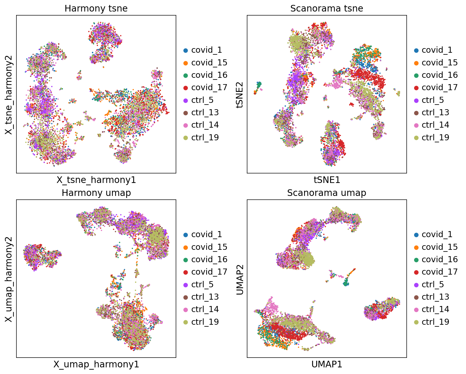
Let’s save the integrated data for further analysis.
# Store this umap and tsne with a new name.
adata2.obsm['X_umap_scanorama'] = adata2.obsm['X_umap']
adata2.obsm['X_tsne_scanorama'] = adata2.obsm['X_tsne']

#save to file, now contains all integrations except the combat one.
save_file = './data/covid/results/scanpy_covid_qc_dr_int.h5ad'
adata2.write_h5ad(save_file)
7 Overview all methods
Now we will plot UMAPS with all three integration methods side by side.
fig, axs = plt.subplots(2, 3, figsize=(10,8),constrained_layout=True)
sc.pl.umap(adata, color="sample", title="Uncorrected", ax=axs[0,0], show=False)
sc.pl.embedding(adata2, 'X_umap_bbknn', color="sample", title="BBKNN", ax=axs[0,1], show=False)
sc.pl.umap(adata_combat, color="sample", title="Combat", ax=axs[0,2], show=False)
sc.pl.embedding(adata2, 'X_umap_harmony', color="sample", title="Harmony", ax=axs[1,0], show=False)
sc.pl.umap(adata2, color="sample", title="Scanorama", ax=axs[1,1], show=False)
<Axes: title={'center': 'Scanorama'}, xlabel='UMAP1', ylabel='UMAP2'>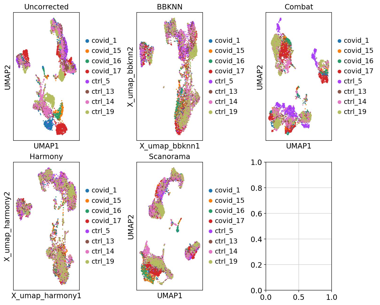
Discuss
Look at the different integration results, which one do you think looks the best? How would you motivate selecting one method over the other? How do you think you could best evaluate if the integration worked well?
8 Extra task
Have a look at the documentation for BBKNN
Try changing some of the parameteres in BBKNN, such as distance metric, number of PCs and number of neighbors. How does the results change with different parameters? Can you explain why?
9 Session info
Click here
sc.logging.print_versions()-----
anndata 0.10.8
scanpy 1.10.3
-----
PIL 11.1.0
annoy NA
asttokens NA
bbknn 1.6.0
cffi 1.17.1
colorama 0.4.6
comm 0.2.2
cycler 0.12.1
cython_runtime NA
dateutil 2.9.0.post0
debugpy 1.8.12
decorator 5.1.1
exceptiongroup 1.2.2
executing 2.1.0
fbpca NA
h5py 3.12.1
harmonypy 0.0.10
igraph 0.11.6
intervaltree NA
ipykernel 6.29.5
jedi 0.19.2
joblib 1.4.2
kiwisolver 1.4.7
legacy_api_wrap NA
leidenalg 0.10.2
llvmlite 0.43.0
matplotlib 3.9.2
matplotlib_inline 0.1.7
mpl_toolkits NA
natsort 8.4.0
numba 0.60.0
numpy 1.26.4
packaging 24.2
pandas 1.5.3
parso 0.8.4
patsy 1.0.1
pickleshare 0.7.5
platformdirs 4.3.6
prompt_toolkit 3.0.50
psutil 6.1.1
pure_eval 0.2.3
pycparser 2.22
pydev_ipython NA
pydevconsole NA
pydevd 3.2.3
pydevd_file_utils NA
pydevd_plugins NA
pydevd_tracing NA
pygments 2.19.1
pynndescent 0.5.13
pyparsing 3.2.1
pytz 2024.2
scanorama 1.7.4
scipy 1.14.1
session_info 1.0.0
six 1.17.0
sklearn 1.6.1
sortedcontainers 2.4.0
sparse 0.15.5
stack_data 0.6.3
texttable 1.7.0
threadpoolctl 3.5.0
torch 2.5.1.post207
torchgen NA
tornado 6.4.2
tqdm 4.67.1
traitlets 5.14.3
typing_extensions NA
umap 0.5.7
wcwidth 0.2.13
yaml 6.0.2
zmq 26.2.0
zoneinfo NA
-----
IPython 8.31.0
jupyter_client 8.6.3
jupyter_core 5.7.2
-----
Python 3.10.16 | packaged by conda-forge | (main, Dec 5 2024, 14:16:10) [GCC 13.3.0]
Linux-6.10.14-linuxkit-x86_64-with-glibc2.35
-----
Session information updated at 2025-02-27 15:15