suppressPackageStartupMessages({
    library(Seurat)
    library(zellkonverter)
    library(Matrix)
    library(ggplot2)
    library(patchwork)
    library(scran)
    library(ComplexHeatmap)
})Go through all the main steps of the pipelines and plot the results side by side.
1 Load data
OBS! Zellkonverter installs conda env with basilisk! Takes a while to run first time!!
path_results <- "data/covid/results"
if (!dir.exists(path_results)) dir.create(path_results, recursive = T)

path_seurat = "../seurat/data/covid/results/"
path_bioc = "../bioc/data/covid/results/"
path_scanpy = "../scanpy/data/covid/results/"

# fetch the files with qc and dimred for each

# seurat
sobj = readRDS(file.path(path_seurat,"seurat_covid_qc_dr_int_cl.rds"))

# bioc
sce = readRDS(file.path(path_bioc,"bioc_covid_qc_dr_int_cl.rds"))
bioc = as.Seurat(sce)

# scanpy
scanpy.sce = readH5AD(file.path(path_scanpy, "scanpy_covid_qc_dr_scanorama_cl.h5ad"))
scanpy = as.Seurat(scanpy.sce, counts = NULL, data = "X") # only have the var.genes data that is scaled.
2 Umaps
wrap_plots(
    DimPlot(sobj, group.by = "orig.ident") + NoAxes() + ggtitle("Seurat"),
    DimPlot(bioc, group.by = "sample") + NoAxes() + ggtitle("Bioc"),
    DimPlot(scanpy, group.by = "sample", reduction = "X_umap_uncorr") + NoAxes() + ggtitle("Scanpy"),
    ncol = 3
)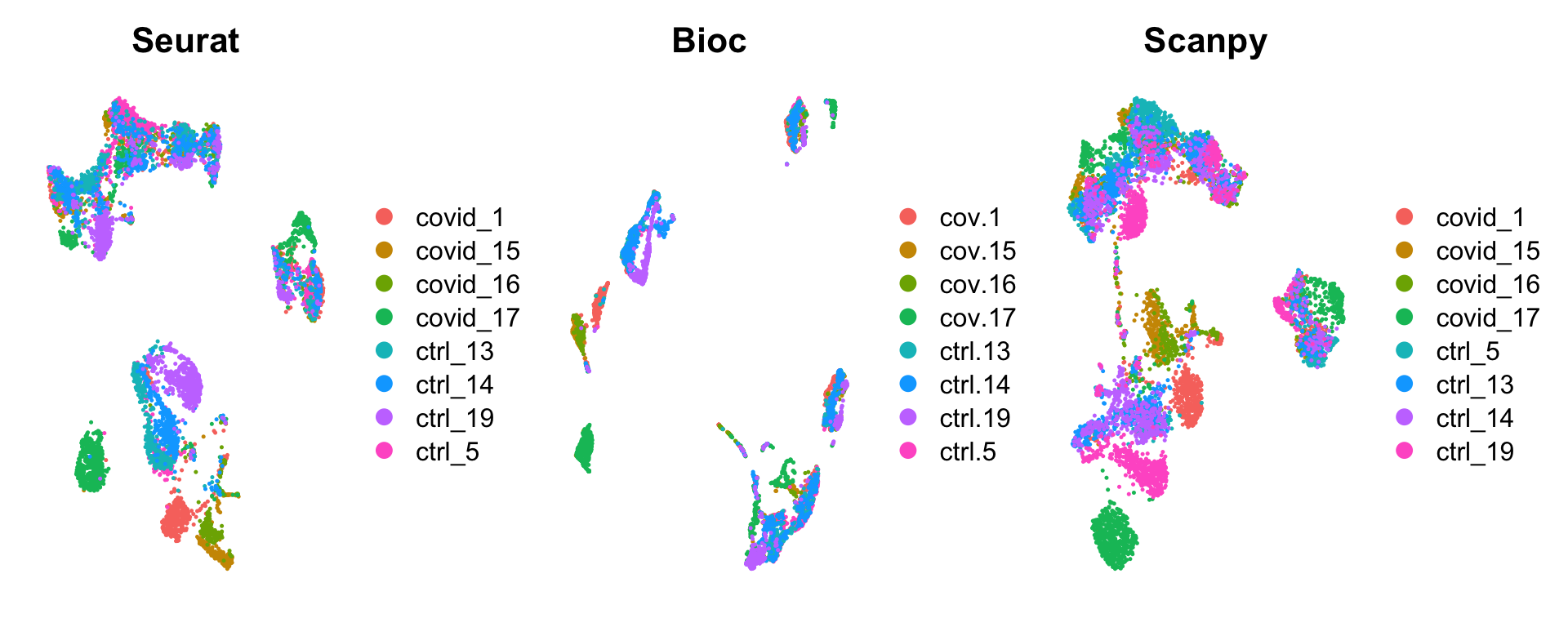
Settings for umap differs, especially on number of neighbors:
Seurat
- dims = 1:30,
- n.neighbors = 30,
- n.epochs = 200,
- min.dist = 0.3,
- learning.rate = 1,
- spread = 1
Bioc
- n_dimred = 30,
- n_neighbors = 15,
- spread = 1,
- min_dist = 0.01,
- n_epchs = 200
Scanpy
- does not use the umap algorithm for neigbors, feeds the KNN to the umap function.
- n_pcs = 30,
- n_neighbors = 20,
- min_dist=0.5,
- spread=1.0,
3 Doublet predictions
In all 3 pipelines we run the filtering of cells in the exact same way, but doublet detection is different.
- In Seurat -
DoubletFinderwith predefined 4% doublets, all samples together. - In Scanpy -
Scrublet, done per batch. No predefined cutoff. - In Bioc -
scDblFinder- default cutoffs, no batch separation.
cat("Seurat: ", dim(sobj),"\n")Seurat: 18854 7134 cat("Bioc: ", dim(bioc),"\n")Bioc: 18854 6830 cat("Scanpy: ", dim(scanpy),"\n")Scanpy: 19468 7222 Highest number of cells filtered with Bioc. Lowest with scanpy.
Cell names are different in all 3, have to make a conversion to match them.
- Seurat has the sample name merged to cell name.
- Scanpy has sample number after cell name.
- Bioc has just cell name.
meta.seurat = sobj@meta.data
meta.scanpy = scanpy@meta.data
meta.bioc = bioc@meta.data

meta.bioc$cell = rownames(meta.bioc)
meta.scanpy$cell = sapply(rownames(meta.scanpy), function(x) substr(x,1,nchar(x)-2))
meta.seurat$cell = unlist(lapply(strsplit(rownames(meta.seurat),"_"), function(x) x[3]))
Visualize overlap of cells using an UpSet plot in the ComplexHeatmap package.
l = list(seurat = meta.seurat$cell, bioc = meta.bioc$cell, scanpy = meta.scanpy$cell)

cmat = make_comb_mat(l)
print(cmat)
A combination matrix with 3 sets and 7 combinations.
ranges of combination set size: c(14, 6616).
mode for the combination size: distinct.
sets are on rows.
Combination sets are:
seurat bioc scanpy code size
x x x 111 6616
x x 110 38
x x 101 408
x x 011 162
x 100 72
x 010 14
x 001 36
Sets are:
set size
seurat 7134
bioc 6830
scanpy 7222UpSet(cmat)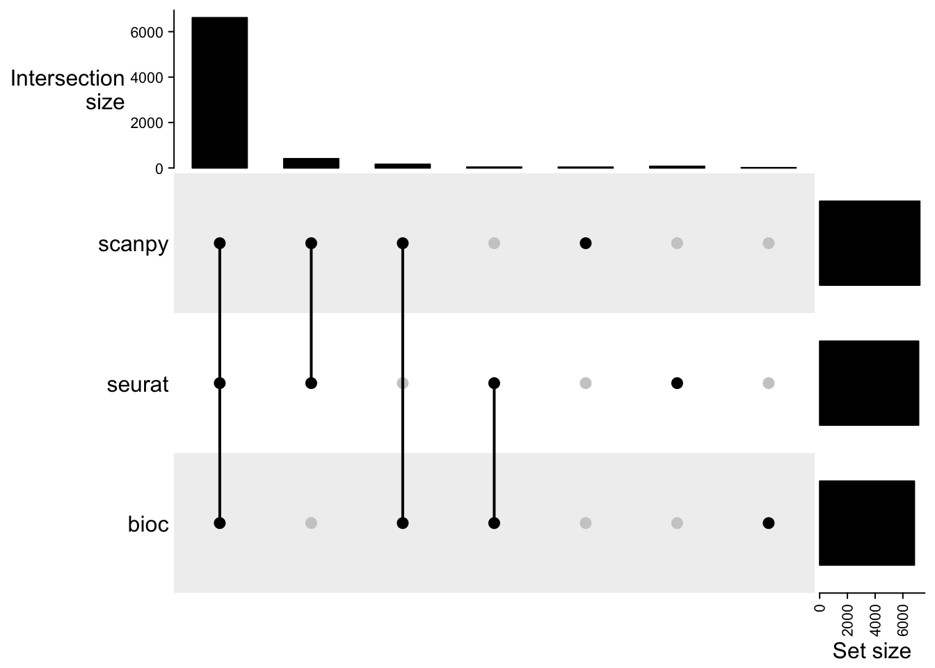
3.1 Doublet scores
Create one dataset with the cells that are present in all samples. Also add in umap from all 3 pipelines.
in.all = intersect(intersect(meta.scanpy$cell, meta.seurat$cell), meta.bioc$cell)

tmp1 = meta.bioc[match(in.all, meta.bioc$cell),]
colnames(tmp1) = paste0(colnames(tmp1),"_bioc")
tmp2 = meta.scanpy[match(in.all, meta.scanpy$cell),]
colnames(tmp2) = paste0(colnames(tmp2),"_scpy")

all = sobj[,match(in.all, meta.seurat$cell)]

meta.all = cbind(all@meta.data, tmp1,tmp2)
all@meta.data = meta.all

Reductions(all)
[1] "pca" "umap" "tsne"
[4] "UMAP10_on_PCA" "UMAP_on_ScaleData" "integrated_cca"
[7] "umap_cca" "tsne_cca" "harmony"
[10] "umap_harmony" "scanorama" "scanoramaC"
[13] "umap_scanorama" "umap_scanoramaC" tmp = bioc@reductions$UMAP_on_PCA@cell.embeddings[match(in.all, meta.bioc$cell),]
rownames(tmp) = colnames(all)
all[["umap_bioc"]] = CreateDimReducObject(tmp, key = "umapbioc_", assay = "RNA")
tmp = scanpy@reductions$X_umap_uncorr@cell.embeddings[match(in.all, meta.scanpy$cell),]
rownames(tmp) = colnames(all)
all[["umap_scpy"]] = CreateDimReducObject(tmp, key = "umapscpy_", assay = "RNA")
Reductions(all) [1] "pca" "umap" "tsne"
[4] "UMAP10_on_PCA" "UMAP_on_ScaleData" "integrated_cca"
[7] "umap_cca" "tsne_cca" "harmony"
[10] "umap_harmony" "scanorama" "scanoramaC"
[13] "umap_scanorama" "umap_scanoramaC" "umap_bioc"
[16] "umap_scpy" wrap_plots(
FeatureScatter(all, "pANN_0.25_0.09_297","scDblFinder.score_bioc"),
FeatureScatter(all, "pANN_0.25_0.09_297","doublet_scores_scpy"),
FeatureScatter(all, "scDblFinder.score_bioc","doublet_scores_scpy"),
ncol = 3
) + plot_layout(guides = "collect")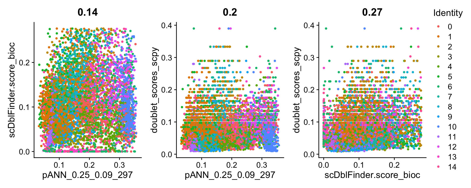
Highest correlation for the doublet scores in Scrublet and scDblFinder, but still only 0.27 in correlation.
wrap_plots(
  FeaturePlot(all, reduction = "umap", features = "pANN_0.25_0.09_297") + NoAxes(),
  FeaturePlot(all, reduction = "umap", features = "scDblFinder.score_bioc") + NoAxes(),
  FeaturePlot(all, reduction = "umap", features = "doublet_scores_scpy") + NoAxes(),
  FeaturePlot(all, reduction = "umap_bioc", features = "pANN_0.25_0.09_297") + NoAxes(),
  FeaturePlot(all, reduction = "umap_bioc", features = "scDblFinder.score_bioc") + NoAxes(),
  FeaturePlot(all, reduction = "umap_bioc", features = "doublet_scores_scpy") + NoAxes(),
  FeaturePlot(all, reduction = "umap_scpy", features = "pANN_0.25_0.09_297") + NoAxes(),
  FeaturePlot(all, reduction = "umap_scpy", features = "scDblFinder.score_bioc") + NoAxes(),
  FeaturePlot(all, reduction = "umap_scpy", features = "doublet_scores_scpy") + NoAxes(),
  ncol = 3
) + plot_layout(guides = "collect")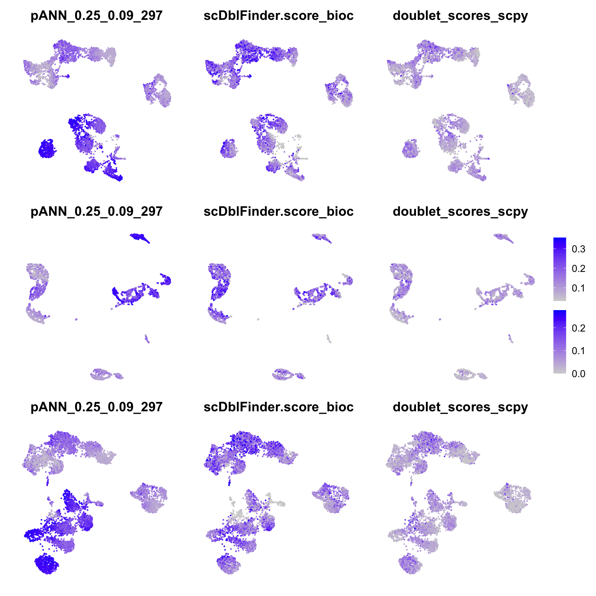
It seems like the DoubletFinder scores are mainly high in the monocyte populations, while it is more mixed in the other 2 methods.
4 Cell cycle
Cell cycle predictions are done in a similar way for Seurat and Scanpy using module scores, while in Bioc we are using Cyclone.
Visualize the phase predictions onto the Seurat umap.
table(all$Phase)
  G1  G2M    S
2890 1531 2195 table(all$phase_bioc)
  G1  G2M    S
3829 749 1553 table(all$phase_scpy)
  G1  G2M    S
5056 74 1486 wrap_plots(
DimPlot(all, group.by = "Phase") + NoAxes(),
DimPlot(all, group.by = "phase_bioc") + NoAxes(),
DimPlot(all, group.by = "phase_scpy") + NoAxes(),
ncol = 3
) + plot_layout(guides = "collect")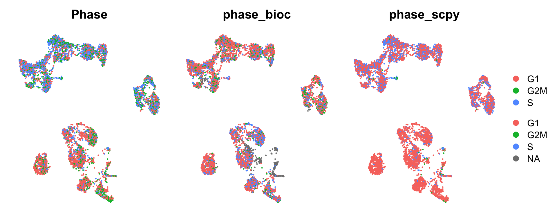
In seurat, most T/B-cells look like cycling. With bioc, more mixed. With scanpy also more in B/T-cells, but much more G1 prediction.
Plot the scores.
cc.scores = c("S.Score", "G2M.Score","G1.score_bioc", "G2M.score_bioc", "S.score_bioc","S_score_scpy", "G2M_score_scpy")


# copied from pairs help section.
panel.cor <- function(x, y, digits = 2, prefix = "", cex.cor, ...) {
    usr <- par("usr")
    on.exit(par(usr))
    par(usr = c(0, 1, 0, 1))
    nas = is.na(x) | is.na(y)
    Cor <- cor(x[!nas], y[!nas], method = "spearman") # Remove abs function if desired
    txt <- paste0(prefix, format(c(Cor, 0.123456789), digits = digits)[1])
    if(missing(cex.cor)) {
        cex.cor <- 0.4 / strwidth(txt)
    }
    text(0.5, 0.5, txt,
         cex = 1 + cex.cor)
}

pairs(all@meta.data[,cc.scores], a.action = na.omit,
      upper.panel = panel.cor,    # Correlation panel
      lower.panel = panel.smooth)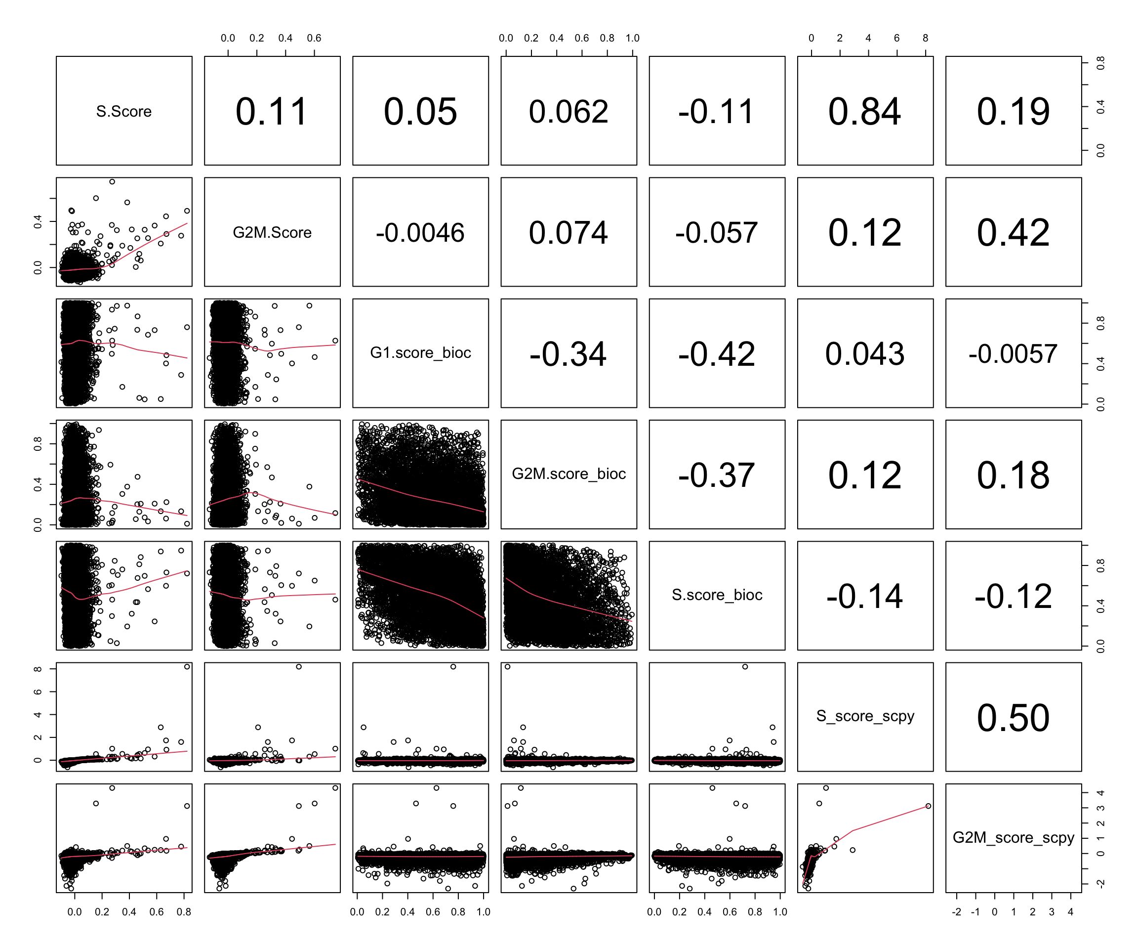
Use spearman cor as the distributions are very different
- S and G2M scores in Scanpy and Seurat are correlated to eachother
- S vs G2M are also correlated.
- In BioC all scores are anticorrelated.
5 Variable features
In Seurat, FindVariableFeatures is not batch aware unless the data is split into layers by samples, here we have the variable genes created with layers. In Bioc modelGeneVar we used sample as a blocking parameter, e.g calculates the variable genes per sample and combines the variances. Similar in scanpy we used the samples as batch_key.
hvgs = list()
hvgs$seurat = VariableFeatures(sobj)
hvgs$bioc = sce@metadata$hvgs
# scanpy has no strict number on selection, instead uses dispersion cutoff. So select instead top 2000 dispersion genes.
tmp = rowData(scanpy.sce)
hvgs_scanpy = rownames(tmp)[tmp$highly_variable]
hvgs$scanpy = rownames(tmp)[order(tmp$dispersions_norm, decreasing = T)][1:2000]

cmat = make_comb_mat(hvgs)
print(cmat)
A combination matrix with 3 sets and 7 combinations.
ranges of combination set size: c(245, 869).
mode for the combination size: distinct.
sets are on rows.
Combination sets are:
seurat bioc scanpy code size
x x x 111 607
x x 110 279
x x 101 245
x x 011 344
x 100 869
x 010 770
x 001 804
Sets are:
set size
seurat 2000
bioc 2000
scanpy 2000UpSet(cmat)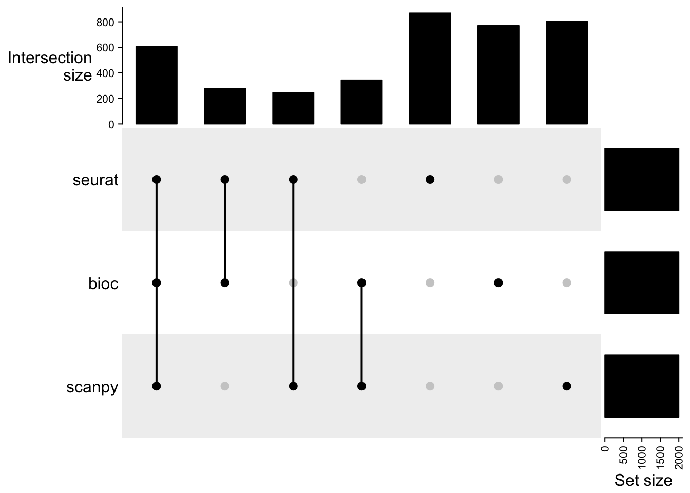
Surprisingly low overlap between the methods and many genes that are unique to one pipeline. With discrepancies in the doublet filtering the cells used differ to some extent, but otherwise the variation should be similar. Even if it is estimated in different ways.
Is the differences more due to the combination of ranks/dispersions or also found within a single dataset?
Only Seurat have the dispersions for each individual dataset stored in the object.
Explore more in the comparison_hvg.qmd script.
6 Integrations
reductions = c("umap","umap_cca", "umap_harmony",  "umap_scanorama",    "umap_scanoramaC", "umap_bioc",  "umap_bioc_mnn", "umap_bioc_harmony", "umap_bioc_scanorama", "umap_scpy","umap_scpy_bbknn", "umap_scpy_scanorama", "umap_scpy_harmony"   )

tmp = bioc@reductions$UMAP_on_MNN@cell.embeddings[match(in.all, meta.bioc$cell),]
rownames(tmp) = colnames(all)
all[["umap_bioc_mnn"]] = CreateDimReducObject(tmp, key = "umapbiocmnn_", assay = "RNA")

tmp = bioc@reductions$UMAP_on_Harmony@cell.embeddings[match(in.all, meta.bioc$cell),]
rownames(tmp) = colnames(all)
all[["umap_bioc_harmony"]] = CreateDimReducObject(tmp, key = "umapbiocharmony_", assay = "RNA")

tmp = bioc@reductions$UMAP_on_Scanorama@cell.embeddings[match(in.all, meta.bioc$cell),]
rownames(tmp) = colnames(all)
all[["umap_bioc_scanorama"]] = CreateDimReducObject(tmp, key = "umapbioscanorama_", assay = "RNA")

tmp = scanpy@reductions$X_umap_bbknn@cell.embeddings[match(in.all, meta.scanpy$cell),]
rownames(tmp) = colnames(all)
all[["umap_scpy_bbknn"]] = CreateDimReducObject(tmp, key = "umapscpybbknn_", assay = "RNA")

tmp = scanpy@reductions$X_umap_scanorama@cell.embeddings[match(in.all, meta.scanpy$cell),]
rownames(tmp) = colnames(all)
all[["umap_scpy_scanorama"]] = CreateDimReducObject(tmp, key = "umapscpyscanorama_", assay = "RNA")

tmp = scanpy@reductions$X_umap_harmony@cell.embeddings[match(in.all, meta.scanpy$cell),]
rownames(tmp) = colnames(all)
all[["umap_scpy_harmony"]] = CreateDimReducObject(tmp, key = "umapscpyharmony_", assay = "RNA")
plotlist = lapply(reductions, function(x) DimPlot(all, reduction = x, group.by = "orig.ident") + NoAxes() + ggtitle(x))
wrap_plots(
plotlist,
ncol = 4
) + plot_layout(guides = "collect")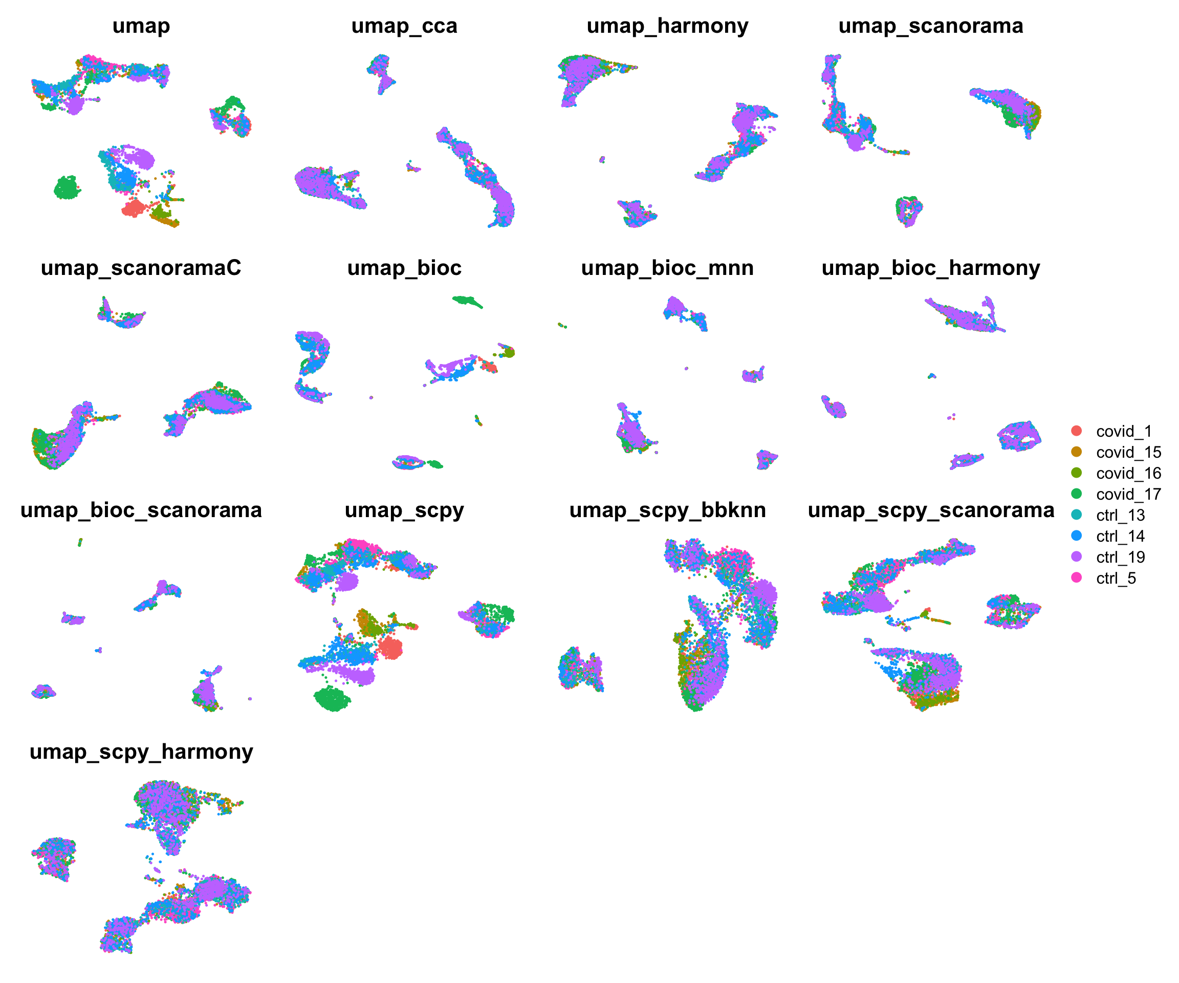
6.1 Clustering on integrations
Run clustering on each of the integrations but with same method. Use Seurat, with 30 first components, k=30, and louvain with a few different resolutions.
For BBKNN the full integration matrix is not in the reductions, skip for now.
# all seurat integrations.

integrations = list(
  seu_cca = "integrated_cca",
  seu_harm = "harmony",
  seu_scan = "scanorama",
  seu_scanC = "scanoramaC"
)
res = c(0.4,0.6,0.8,1.0)

for (i in 1:length(integrations)){
  sname = names(integrations)[i]
  sobj = FindNeighbors(sobj, reduction = integrations[[sname]], dims = 1:30, verbose = F)
  for (r in res){
    sobj = FindClusters(sobj, resolution = r, cluster.name = paste(sname,r,sep="_"), verbose = F)
  }
}

meta.clust = sobj@meta.data[,grepl("^seu_", colnames(sobj@meta.data))]
meta.clust = meta.clust[match(in.all, meta.seurat$cell),]

# all bioc
integrations = list(
  bio_mnn = "MNN",
  bio_harm = "harmony",
  bio_scan = "Scanorama"
)

for (i in 1:length(integrations)){
  sname = names(integrations)[i]
  bioc = FindNeighbors(bioc, reduction = integrations[[sname]], dims = 1:30, verbose = F)
  for (r in res){
    bioc = FindClusters(bioc, resolution = r, cluster.name = paste(sname,r,sep="_"), verbose = F)
  }
}

tmp = bioc@meta.data[,grepl("^bio_", colnames(bioc@meta.data))]
tmp = tmp[match(in.all, meta.bioc$cell),]
meta.clust = cbind(tmp, meta.clust)

# all scanpy
integrations = list(
  scpy_harm = "X_pca_harmony",
  scpy_scan = "Scanorama"
)

for (i in 1:length(integrations)){
  sname = names(integrations)[i]
  scanpy = FindNeighbors(scanpy, reduction = integrations[[sname]], dims = 1:30, verbose = F)
  for (r in res){
    scanpy = FindClusters(scanpy, resolution = r, cluster.name = paste(sname,r,sep="_"), verbose = F)
  }
}

tmp = scanpy@meta.data[,grepl("^scpy_", colnames(scanpy@meta.data))]
tmp = tmp[match(in.all, meta.scanpy$cell),]
meta.clust = cbind(tmp, meta.clust)
Calculate adjusted Rand index, with mclust package.
ari = mat.or.vec(ncol(meta.clust), ncol(meta.clust))

for (i in 1:ncol(meta.clust)){
  for (j in 1:ncol(meta.clust)){
  ari[i,j] = mclust::adjustedRandIndex(meta.clust[,i], meta.clust[,j])
  }
}
rownames(ari) = colnames(meta.clust)
colnames(ari) = colnames(meta.clust)

annot = data.frame(Reduce(rbind,strsplit(colnames(meta.clust), "_")))
colnames(annot) = c("Pipe", "Integration", "Resolution")
rownames(annot) = colnames(meta.clust)
nclust = apply(meta.clust, 2, function(x) length(unique(x)))
annot$nClust = nclust
pheatmap::pheatmap(ari, annotation_row = annot)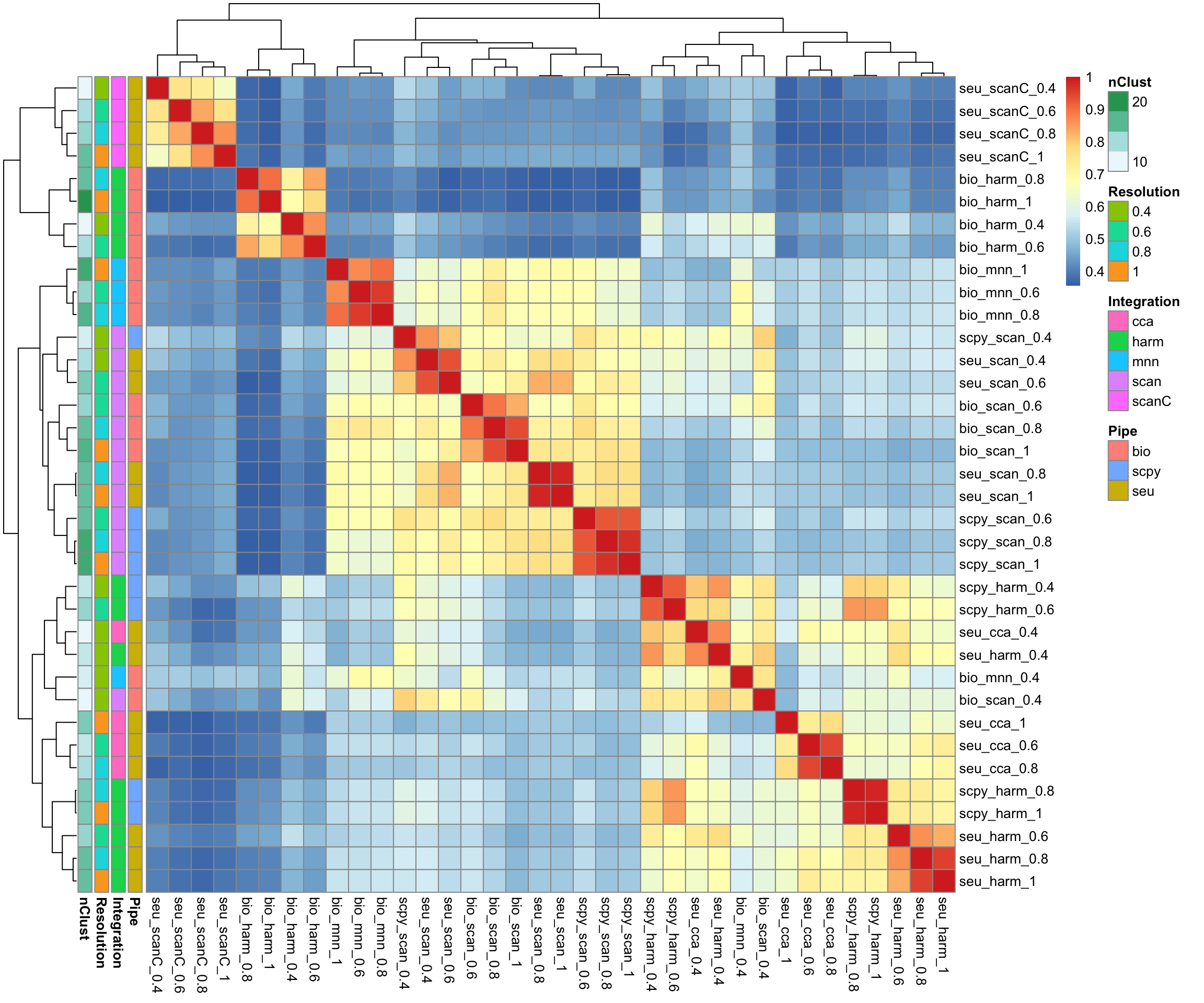
All the scanorama ones are similar, except for the one with counts. Harmony on the bioc object also stands out as quite different.
Number of clusters per method:
nclust = apply(meta.clust, 2, function(x) length(unique(x)))
par(mar = c(3,10,3,3))
barplot(nclust, horiz=T, las=2, cex.names=0.6)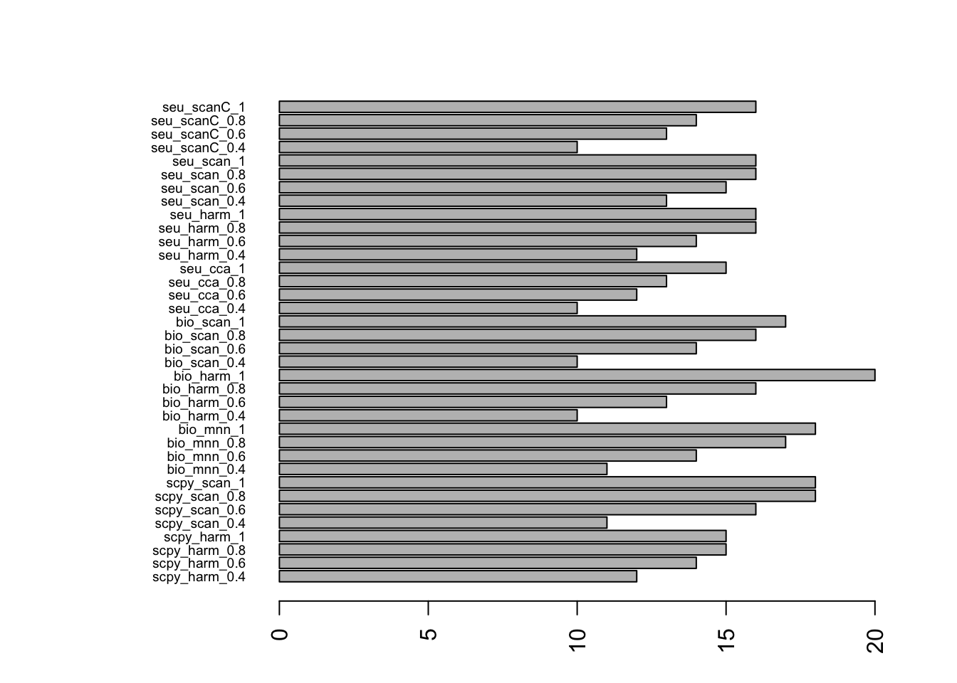
For similar number of clusters, select the ones with nclust close to 15.
selCl = c("scpy_harm_0.8","scpy_scan_0.6","bio_mnn_0.8","bio_harm_0.8","bio_scan_0.8","seu_cca_1","seu_harm_0.8","seu_scan_0.6","seu_scanC_1")

pheatmap::pheatmap(ari[selCl,selCl], annotation_row = annot[selCl,])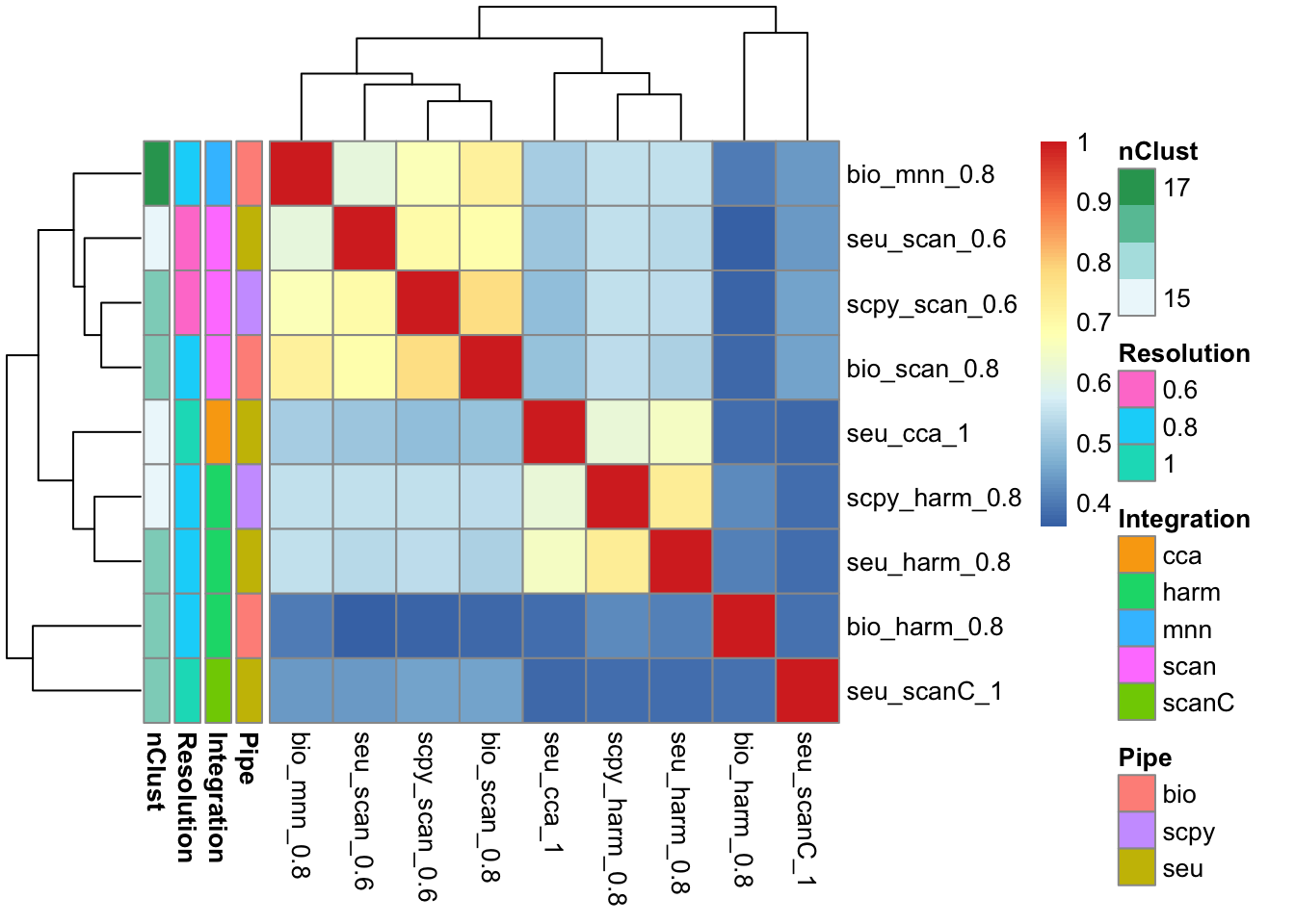
7 Clustering in the exercises
Above, we did the clustering with the same method on the different integrated spaces. Now we will instead explore the integrated clustering from the different pipelines. We still only use the cells that are in common from all 3 toolkits.
The graph clustering is implemented quite differently in the different pipelines.
- Seurat - runs detection on SNN, resolution implemented
- Scanpy - runs detection on KNN, resolution implemented
- Bioc - runs detection on SNN, but different scoring to Seurat, resolution parameter behaves strange. Instead use
kto tweak cluster resolution.
seu.columns = c("RNA_snn_res","kmeans_","hc_")
bioc.columns = c("louvain_","leiden_","hc_","kmeans_")
scpy.columns = c("leiden_","hclust_","kmeans_")


idx = which(rowSums(sapply(seu.columns, grepl, colnames(sobj@meta.data)))>0)
tmp1 = sobj@meta.data[match(in.all, meta.seurat$cell), idx]
colnames(tmp1) = paste0("seur_", colnames(tmp1))

idx = which(rowSums(sapply(bioc.columns, grepl, colnames(bioc@meta.data)))>0)
tmp2 = bioc@meta.data[match(in.all, meta.bioc$cell), idx]
colnames(tmp2) = paste0("bioc_", colnames(tmp2))

meta.clust2 = cbind(tmp1, tmp2)

idx = which(rowSums(sapply(scpy.columns, grepl, colnames(scanpy@meta.data)))>0)
tmp2 = scanpy@meta.data[match(in.all, meta.scanpy$cell), idx]
colnames(tmp2) = paste0("scpy_", colnames(tmp2))

meta.clust2 = cbind(meta.clust2, tmp2)
Group based on adjusted Rand index.
ari = mat.or.vec(ncol(meta.clust2), ncol(meta.clust2))

for (i in 1:ncol(meta.clust2)){
  for (j in 1:ncol(meta.clust2)){
  ari[i,j] = mclust::adjustedRandIndex(meta.clust2[,i], meta.clust2[,j])
  }
}
rownames(ari) = colnames(meta.clust2)
colnames(ari) = colnames(meta.clust2)


m = unlist(lapply(strsplit(colnames(meta.clust2), "_"), function(x) x[2]))
p = unlist(lapply(strsplit(colnames(meta.clust2), "_"), function(x) x[1]))
nc = apply(meta.clust2, 2, function(x) length(unique(x)))

annot = data.frame(Pipe=p, Method=m, nC=nc)
rownames(annot) = colnames(meta.clust2)
pheatmap::pheatmap(ari, annotation_row = annot)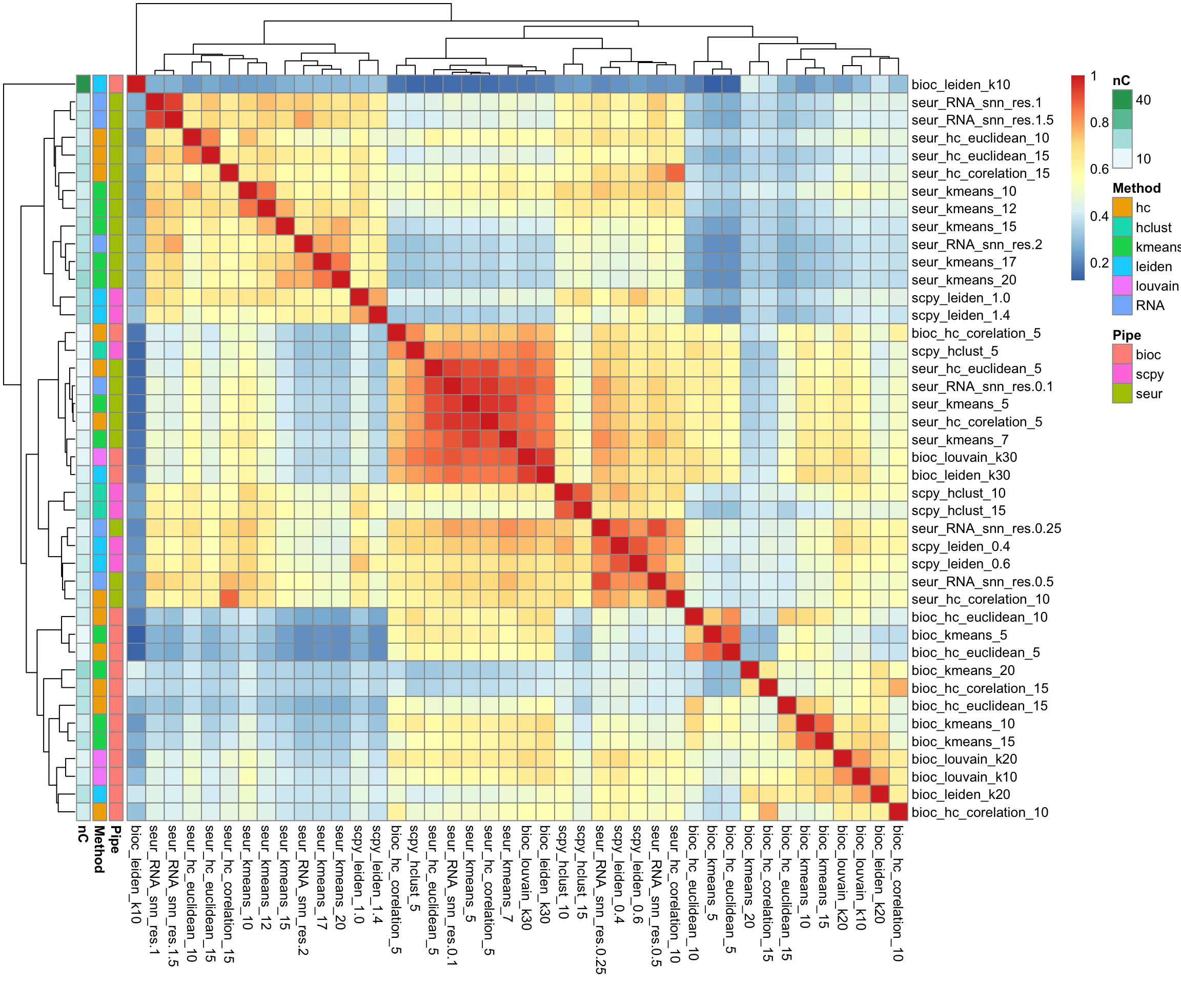
saveRDS(all, "data/covid/results/merged_all.rds")8 Celltype prediction.
Done only for sample ctrl13, load all the results.
sobj = readRDS(file.path(path_seurat, "seurat_covid_qc_dr_int_cl_ct-ctrl13.rds"))

sce = readRDS(file.path(path_bioc, "bioc_covid_qc_dr_int_cl_ct-ctrl13.rds"))
bioc = as.Seurat(sce)
bioc$scmap_cluster = sce$scmap_cluster #for some reason that column dissappears when running as.Seurat.

scanpy.sce = readH5AD(file.path(path_scanpy, "scanpy_covid_qc_dr_int_cl_ct-ctrl13.h5ad"))
scanpy = as.Seurat(scanpy.sce, counts = NULL, data = "X")
Merge into one object.
meta.seurat = sobj@meta.data
meta.scanpy = scanpy@meta.data
meta.bioc = bioc@meta.data

meta.bioc$cell = rownames(meta.bioc)
meta.scanpy$cell = sapply(rownames(meta.scanpy), function(x) substr(x,1,nchar(x)-2))
meta.seurat$cell = unlist(lapply(strsplit(rownames(meta.seurat),"_"), function(x) x[3]))

in.all = intersect(intersect(meta.scanpy$cell, meta.seurat$cell), meta.bioc$cell)

tmp1 = meta.bioc[match(in.all, meta.bioc$cell),]
colnames(tmp1) = paste0(colnames(tmp1),"_bioc")
tmp2 = meta.scanpy[match(in.all, meta.scanpy$cell),]
colnames(tmp2) = paste0(colnames(tmp2),"_scpy")

all = sobj[,match(in.all, meta.seurat$cell)]

meta.all = cbind(all@meta.data, tmp1,tmp2)
all@meta.data = meta.all
Celltype predictions:
Seurat
predicted.id-TransferDatasingler.immune- singleR withDatabaseImmuneCellExpressionDatasingler.hpca- singleR withHumanPrimaryCellAtlasDatasingler.ref- singleR with own ref.predicted.celltype.l1,predicted.celltype.l2,predicted.celltype.l3- Azimuth predictions at different levels.
Bioc
scmap_cluster- scMap with clusters in ref datascmap_cell- scMap with all cells in ref datasingler.immune- singleR withDatabaseImmuneCellExpressionDatasingler.hpca- singleR withHumanPrimaryCellAtlasDatasingler.ref- singleR with own ref.
Scanpy
label_trans- label transfer with scanoramalouvain- bbknnpredicted_labels,majority_voting- celltypist “Immune_All_High” referencepredicted_labels_ref,majority_voting_ref- celltypist with own reference
all.pred = c("label_trans_scpy",   "louvain_scpy",  "predicted_labels_scpy", "majority_voting_scpy", "predicted_labels_ref_scpy",  "majority_voting_ref_scpy",      "scmap_cluster_bioc", "scmap_cell_bioc",  "singler.immune_bioc", "singler.hpca_bioc",  "singler.ref_bioc", "predicted.id", "singler.immune", "singler.hpca",  "singler.ref", "predicted.celltype.l1", "predicted.celltype.l2", "predicted.celltype.l3")

ct = all@meta.data[,all.pred]

plots = sapply(all.pred, function(x) DimPlot(all, reduction = "umap_harmony", group.by = x) + NoAxes() + ggtitle(x))

wrap_plots(plots[1:9], ncol = 3)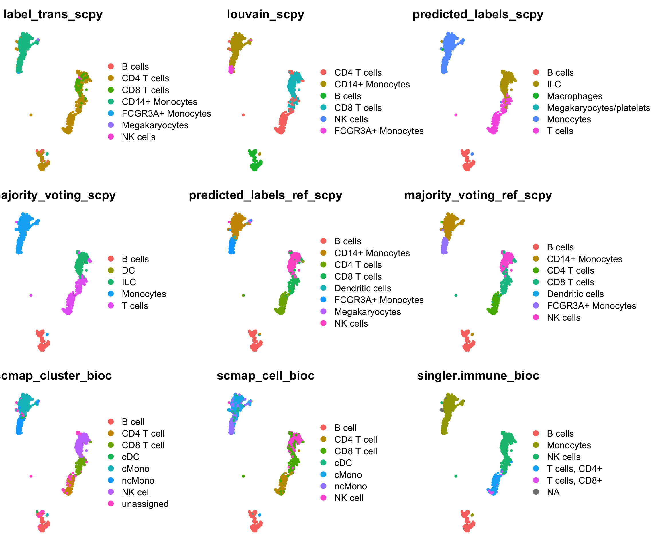
wrap_plots(plots[10:18], ncol = 3)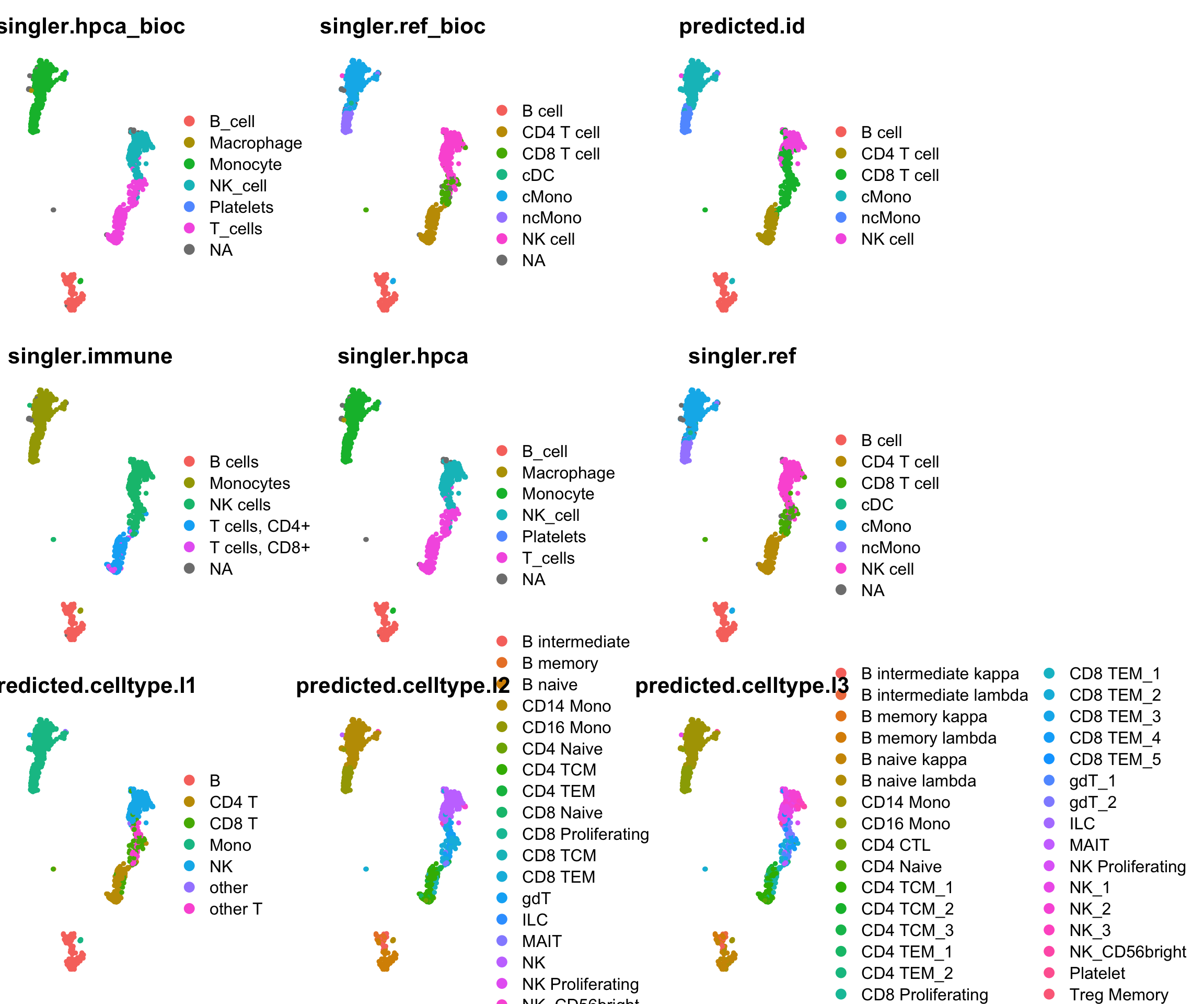
Subset for ones that are using same ref:
ref.pred = c("label_trans_scpy",   "louvain_scpy", "predicted_labels_ref_scpy",  "majority_voting_ref_scpy",      "scmap_cluster_bioc", "scmap_cell_bioc",   "singler.ref_bioc", "predicted.id",  "singler.ref")

lev = sort(unique(unlist(apply(all@meta.data[,ref.pred],2,unique))))
lev = unique(sub("cells","cell",lev))

#"FCGR3A+ Monocytes" -> "ncMono"
#"CD14+ Monocytes" -> "cMono"
#"Dendritic cell" -> "cDC"
lev = lev[!grepl("\\+",lev)]
lev = lev[!grepl("Dendr",lev)]

for (rp in ref.pred){
  tmp = as.character(all@meta.data[,rp])
  tmp = sub("cells","cell",tmp)
  tmp = sub("FCGR3A\\+ Monocytes","ncMono",tmp)
  tmp = sub("CD14\\+ Monocytes","cMono",tmp)
  tmp = sub("Dendritic cell","cDC",tmp)
  tmp[is.na(tmp)] = "unassigned"
  all@meta.data[,paste0(rp,"2")] = factor(tmp,levels = lev)

}

coldef =  RColorBrewer::brewer.pal(9,"Paired")
names(coldef) = lev
plots2 = sapply(paste0(ref.pred,"2"), function(x) DimPlot(all, reduction = "umap_harmony", group.by = x) + NoAxes() + ggtitle(x) + scale_color_manual(values = coldef))


wrap_plots(plots2, ncol = 3) + plot_layout(guides = "collect")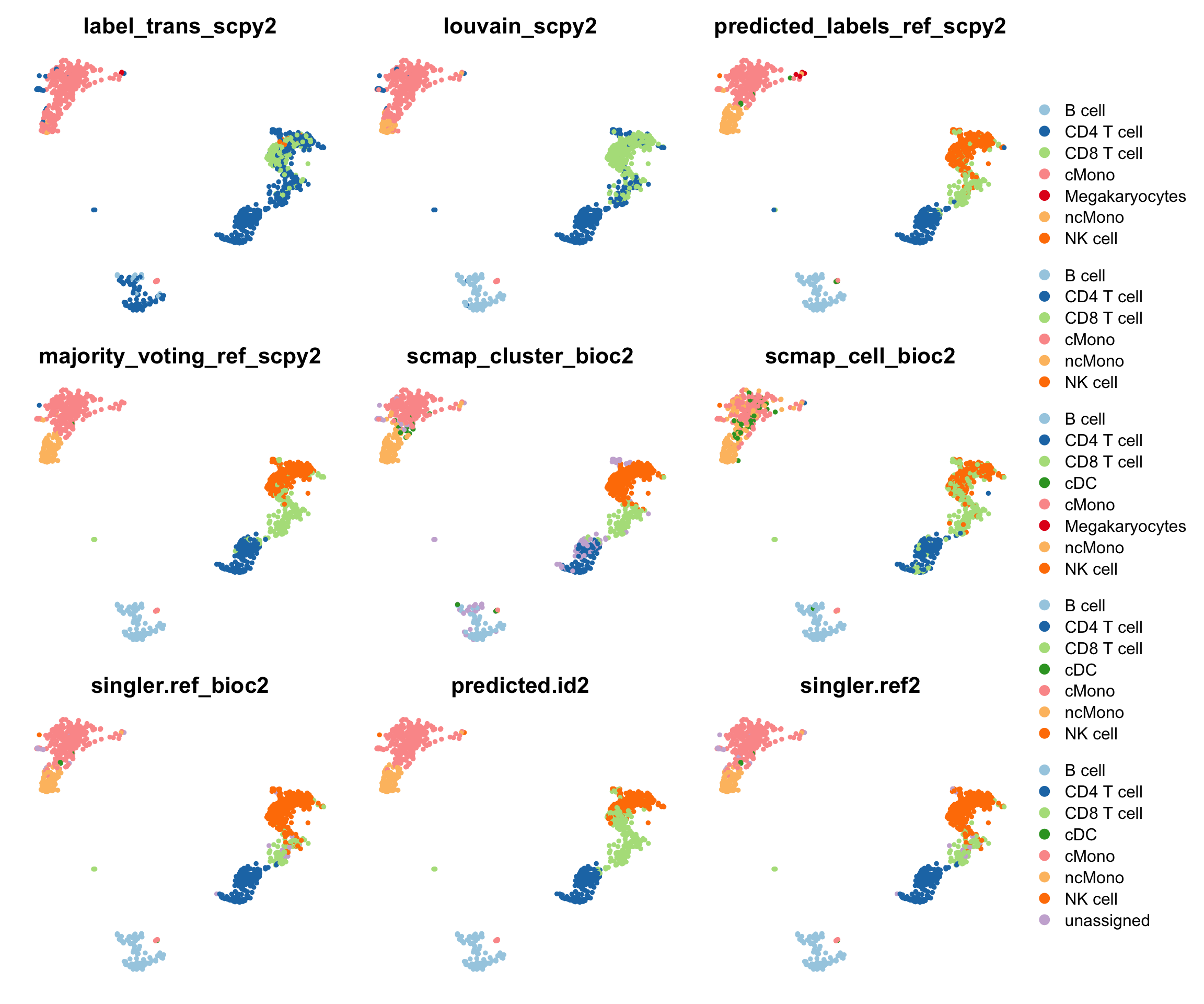
The largest differences in predictions is for CD8T vs NK where the methods make quite different prediction for the cells in between the two celltypes.
ref.pred2 = paste0(ref.pred,"2")

tmp = all@meta.data[,ref.pred2]

counts = sapply(ref.pred2,function(x) table(tmp[,x]))
counts = reshape2::melt(counts)


ggplot(counts, aes(x=Var2, y=value, fill=Var1)) + geom_bar(stat = "identity") + RotatedAxis() 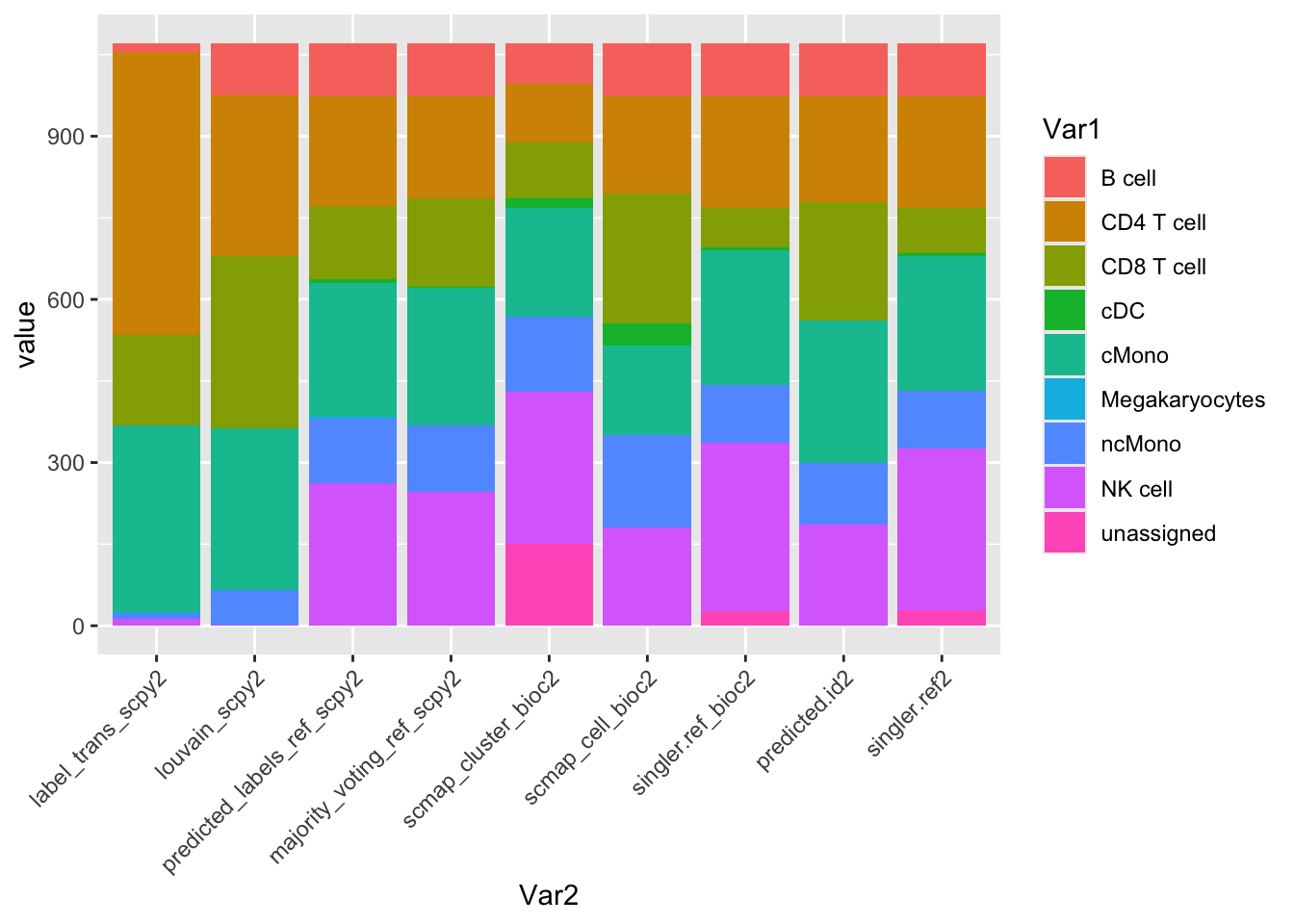
Only singleR and scMap has unassigned cells.
Prediction overlaps, based on ARI.
ari = mat.or.vec(ncol(tmp), ncol(tmp))

for (i in 1:ncol(tmp)){
  for (j in 1:ncol(tmp)){
  ari[i,j] = mclust::adjustedRandIndex(tmp[,i], tmp[,j])
  }
}
rownames(ari) = colnames(tmp)
colnames(ari) = colnames(tmp)

pheatmap::pheatmap(ari)
Celltypist and singleR are quite similar.
9 Session info
Click here
sessionInfo()R version 4.3.3 (2024-02-29)
Platform: x86_64-apple-darwin13.4.0 (64-bit)
Running under: macOS Big Sur ... 10.16
Matrix products: default
BLAS/LAPACK: /Users/asabjor/miniconda3/envs/seurat5_u/lib/libopenblasp-r0.3.28.dylib; LAPACK version 3.12.0
locale:
[1] sv_SE.UTF-8/sv_SE.UTF-8/sv_SE.UTF-8/C/sv_SE.UTF-8/sv_SE.UTF-8
time zone: Europe/Stockholm
tzcode source: system (macOS)
attached base packages:
[1] grid stats4 stats graphics grDevices utils datasets
[8] methods base
other attached packages:
[1] ComplexHeatmap_2.18.0 scran_1.30.0
[3] scuttle_1.12.0 SingleCellExperiment_1.24.0
[5] SummarizedExperiment_1.32.0 Biobase_2.62.0
[7] GenomicRanges_1.54.1 GenomeInfoDb_1.38.1
[9] IRanges_2.36.0 S4Vectors_0.40.2
[11] BiocGenerics_0.48.1 MatrixGenerics_1.14.0
[13] matrixStats_1.5.0 patchwork_1.3.0
[15] ggplot2_3.5.1 Matrix_1.6-5
[17] zellkonverter_1.12.1 Seurat_5.1.0
[19] SeuratObject_5.0.2 sp_2.1-4
loaded via a namespace (and not attached):
[1] RcppAnnoy_0.0.22 splines_4.3.3
[3] later_1.4.1 bitops_1.0-9
[5] filelock_1.0.3 tibble_3.2.1
[7] polyclip_1.10-7 basilisk.utils_1.14.1
[9] fastDummies_1.7.4 lifecycle_1.0.4
[11] doParallel_1.0.17 edgeR_4.0.16
[13] globals_0.16.3 lattice_0.22-6
[15] MASS_7.3-60.0.1 magrittr_2.0.3
[17] limma_3.58.1 plotly_4.10.4
[19] rmarkdown_2.29 yaml_2.3.10
[21] metapod_1.10.0 httpuv_1.6.15
[23] sctransform_0.4.1 spam_2.11-0
[25] spatstat.sparse_3.1-0 reticulate_1.40.0
[27] cowplot_1.1.3 pbapply_1.7-2
[29] RColorBrewer_1.1-3 abind_1.4-5
[31] zlibbioc_1.48.0 Rtsne_0.17
[33] purrr_1.0.2 RCurl_1.98-1.16
[35] circlize_0.4.16 GenomeInfoDbData_1.2.11
[37] ggrepel_0.9.6 irlba_2.3.5.1
[39] listenv_0.9.1 spatstat.utils_3.1-2
[41] pheatmap_1.0.12 goftest_1.2-3
[43] RSpectra_0.16-2 spatstat.random_3.3-2
[45] dqrng_0.3.2 fitdistrplus_1.2-2
[47] parallelly_1.41.0 DelayedMatrixStats_1.24.0
[49] leiden_0.4.3.1 codetools_0.2-20
[51] DelayedArray_0.28.0 shape_1.4.6.1
[53] tidyselect_1.2.1 farver_2.1.2
[55] ScaledMatrix_1.10.0 spatstat.explore_3.3-4
[57] jsonlite_1.8.9 GetoptLong_1.0.5
[59] BiocNeighbors_1.20.0 progressr_0.15.1
[61] iterators_1.0.14 ggridges_0.5.6
[63] survival_3.8-3 foreach_1.5.2
[65] tools_4.3.3 ica_1.0-3
[67] Rcpp_1.0.13-1 glue_1.8.0
[69] gridExtra_2.3 SparseArray_1.2.2
[71] xfun_0.50 dplyr_1.1.4
[73] withr_3.0.2 fastmap_1.2.0
[75] basilisk_1.14.1 bluster_1.12.0
[77] digest_0.6.37 rsvd_1.0.5
[79] R6_2.5.1 mime_0.12
[81] colorspace_2.1-1 Cairo_1.6-2
[83] scattermore_1.2 tensor_1.5
[85] spatstat.data_3.1-4 tidyr_1.3.1
[87] generics_0.1.3 data.table_1.15.4
[89] httr_1.4.7 htmlwidgets_1.6.4
[91] S4Arrays_1.2.0 uwot_0.1.16
[93] pkgconfig_2.0.3 gtable_0.3.6
[95] lmtest_0.9-40 XVector_0.42.0
[97] htmltools_0.5.8.1 dotCall64_1.2
[99] clue_0.3-66 scales_1.3.0
[101] png_0.1-8 spatstat.univar_3.1-1
[103] knitr_1.49 rjson_0.2.23
[105] reshape2_1.4.4 nlme_3.1-165
[107] GlobalOptions_0.1.2 zoo_1.8-12
[109] stringr_1.5.1 KernSmooth_2.23-26
[111] parallel_4.3.3 miniUI_0.1.1.1
[113] pillar_1.10.1 vctrs_0.6.5
[115] RANN_2.6.2 promises_1.3.2
[117] BiocSingular_1.18.0 beachmat_2.18.0
[119] xtable_1.8-4 cluster_2.1.8
[121] evaluate_1.0.1 cli_3.6.3
[123] locfit_1.5-9.10 compiler_4.3.3
[125] rlang_1.1.4 crayon_1.5.3
[127] future.apply_1.11.2 labeling_0.4.3
[129] mclust_6.1.1 plyr_1.8.9
[131] stringi_1.8.4 viridisLite_0.4.2
[133] deldir_2.0-4 BiocParallel_1.36.0
[135] munsell_0.5.1 lazyeval_0.2.2
[137] spatstat.geom_3.3-4 dir.expiry_1.10.0
[139] RcppHNSW_0.6.0 sparseMatrixStats_1.14.0
[141] future_1.34.0 statmod_1.5.0
[143] shiny_1.10.0 ROCR_1.0-11
[145] igraph_2.0.3