suppressPackageStartupMessages({
    library(Seurat)
    library(Matrix)
    library(ggplot2)
    library(patchwork)
    library(scran)
    library(basilisk)
    library(dplyr)
})

devtools::source_url("https://raw.githubusercontent.com/asabjorklund/single_cell_R_scripts/main/overlap_phyper_v2.R")Run different methods of normalization and look at how the distributions look after norm.
- Lognorm with different scale factors.
- SCT with all cells or per sample. How are residuals effected?
- TMM, Quantile.
- Deconvolution
- Pearson residuals in scanpy
1 Load data
path_seurat = "../seurat/data/covid/results/"

# seurat
sobj = readRDS(file.path(path_seurat,"seurat_covid_qc_dr_int_cl.rds"))
sobj
An object of class Seurat
18854 features across 7134 samples within 1 assay
Active assay: RNA (18854 features, 2000 variable features)
17 layers present: counts.covid_1, counts.covid_15, counts.covid_16, counts.covid_17, counts.ctrl_5, counts.ctrl_13, counts.ctrl_14, counts.ctrl_19, scale.data, data.covid_1, data.covid_15, data.covid_16, data.covid_17, data.ctrl_5, data.ctrl_13, data.ctrl_14, data.ctrl_19
14 dimensional reductions calculated: pca, umap, tsne, UMAP10_on_PCA, UMAP_on_ScaleData, integrated_cca, umap_cca, tsne_cca, harmony, umap_harmony, scanorama, scanoramaC, umap_scanorama, umap_scanoramaCThe object has the data split into layers, both counts and data. One single scale.data layer.
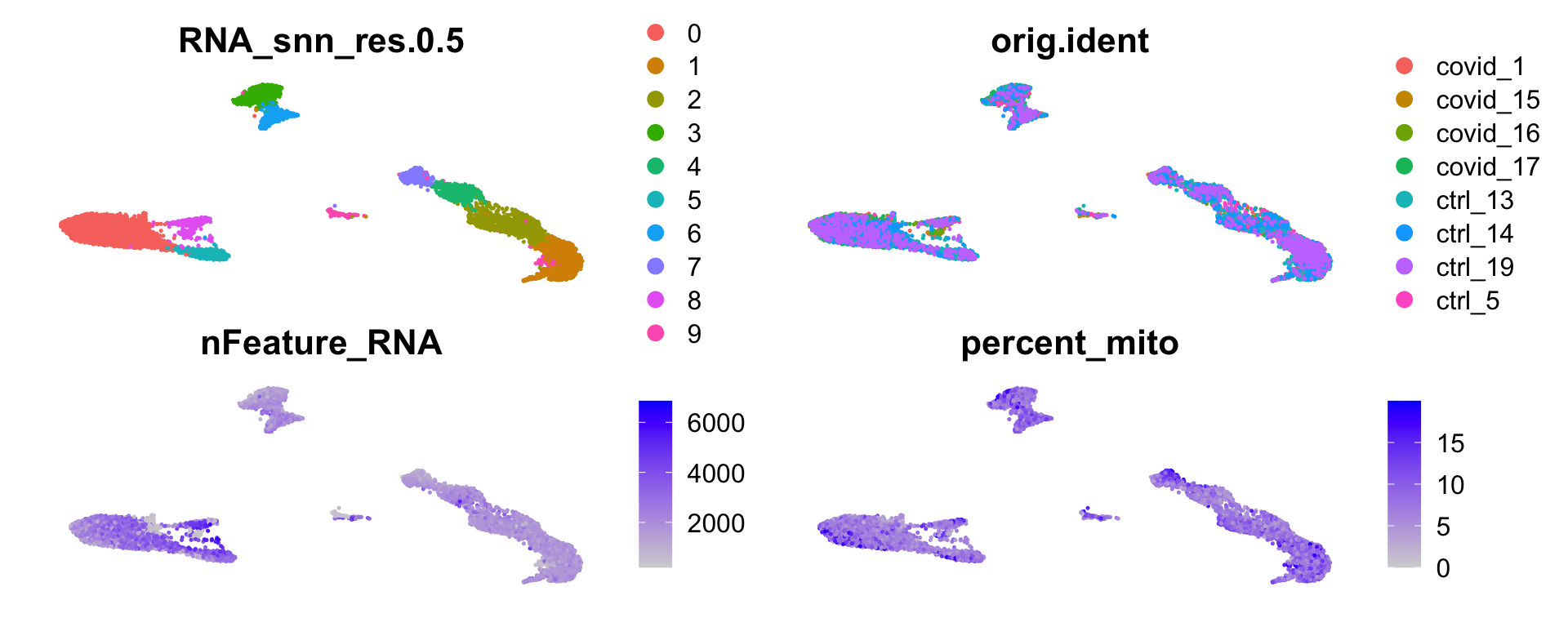
Plot integrated data:
wrap_plots(
    DimPlot(sobj, group.by = "RNA_snn_res.0.5", reduction = "umap_cca") + NoAxes(),
    DimPlot(sobj, group.by = "orig.ident", reduction = "umap_cca") + NoAxes(),
    FeaturePlot(sobj,  "nFeature_RNA", reduction = "umap_cca") + NoAxes(),
    FeaturePlot(sobj,  "percent_mito", reduction = "umap_cca") + NoAxes(),
    ncol = 2
)
sobj = SetIdent(sobj, value = "RNA_snn_res.0.5")
sobj@active.assay = "RNA"
Select a set of variable genes to analyse across all normalizations, 5K genes.
sobj = FindVariableFeatures(sobj, nfeatures = 5000, verbose = F)

hvg = VariableFeatures(sobj)
2 Normalize
2.1 SCT per layer
First, run SCT on each layer, e.g. each sample.
sobj = SCTransform(sobj, new.assay.name = "SCTL", verbose = F)

dim(sobj@assays$SCTL@counts)
[1] 15161 7134dim(sobj@assays$SCTL@data)[1] 15161 7134dim(sobj@assays$SCTL@scale.data)[1] 6545 7134First runs SCT for each layer separately, then creates one merged counts, data, scale.data.
Fewer genes in the SCT counts/data matrix.
vg = list()
for (n in names(sobj@assays$SCTL@SCTModel.list)){
  vg[[n]] = rownames(sobj@assays$SCTL@SCTModel.list[[n]]@feature.attributes)[sobj@assays$SCTL@SCTModel.list[[n]]@feature.attributes$genes_log_gmean_step1]
}

o = overlap_phyper2(vg,vg, bg = nrow(sobj@assays$RNA))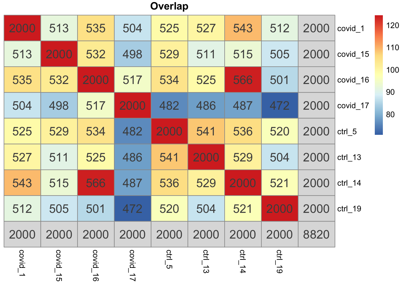
all.vg = unique(unlist(vg))

length(all.vg)
[1] 8820dim(sobj@assays$SCTL@scale.data)[1] 6545 7134sum(rownames(sobj@assays$SCTL@scale.data) %in% all.vg)[1] 4437Total variable genes from each dataset is more than the size of scale.data. The function first runs SCT for each dataset, then runs Seurat VariableFeatures on each object. and takes the union!
# from the seurat function:
      vf.list <- lapply(X  = sct.assay.list, FUN = function(object.i) VariableFeatures(object = object.i))
      variable.features.union <- Reduce(f = union, x = vf.list)
Those genes are used to calculate the residuals in scale.data. Still, among those genes, only 4437 are among the first set of 5000 variable genes.
Calculate residuals for all genes:
sobj = PrepSCTFindMarkers(sobj, assay = "SCTL")
#, anchor.features = intersect(rownames(sobj), hvg))$s
2.2 Annotation
Merge the layers and run all normalization with all genes together. Filter genes with less than 5 cells.
sobj@active.assay = "RNA"
sobj <- JoinLayers(object = sobj, layers = c("data","counts"))

# remove genes with less than 5 cells.
nC = rowSums(sobj@assays$RNA@layers$counts > 0)
sobj = sobj[nC>4,]
sobj = NormalizeData(sobj, verbose = F)

# add the normalized to a list
ndata = list()
C = sobj@assays$RNA@layers$counts
rownames(C) = rownames(sobj)
colnames(C) = colnames(sobj)
ndata$counts = C
D = sobj@assays$RNA@layers$data
rownames(D) = rownames(sobj)
colnames(D) = colnames(sobj)
ndata$lognorm10k = D


# also add in the SCTL data
ndata$sctl_counts = sobj@assays$SCTL@counts
ndata$sctl_data = sobj@assays$SCTL@data
ndata$sctl_scaledata = sobj@assays$SCTL@scale.data
Add celltype annotation from Azimuth. Define as broad celltypes based on the clusters for visualization.
celltype.file = "data/celltype_azimuth.csv"
if (file.exists(celltype.file)){
  ct = read.csv(celltype.file, row.names = 1)
  sobj$celltype = ct$celltype
  sobj$predicted.celltype.l1 = ct$predicted.celltype.l1
}else {
  library(Azimuth)
  sobj <- RunAzimuth(sobj, reference = "pbmcref")
  annot = list("0"="Mono","5"="Mono","8"="Other","9"="Mix","3"="BC","6"="BC","1"="NK","2"="TC","4"="TC", "7"="TC")
  sobj$celltype = unname(unlist(annot[as.character(sobj@active.ident)]))
  ct = sobj@meta.data[,c("celltype","predicted.celltype.l1")]
  write.csv(ct, file=celltype.file)

}
p1 = DimPlot(sobj, label = T, reduction = "umap_cca")  + NoAxes()
p2 = DimPlot(sobj, reduction = "umap_cca", group.by = "predicted.celltype.l1", label = T) + NoAxes()

p3 = DimPlot(sobj, reduction = "umap_cca", group.by = "celltype", label = T) + NoAxes()
wrap_plots(p1,p2,p3, ncol=2)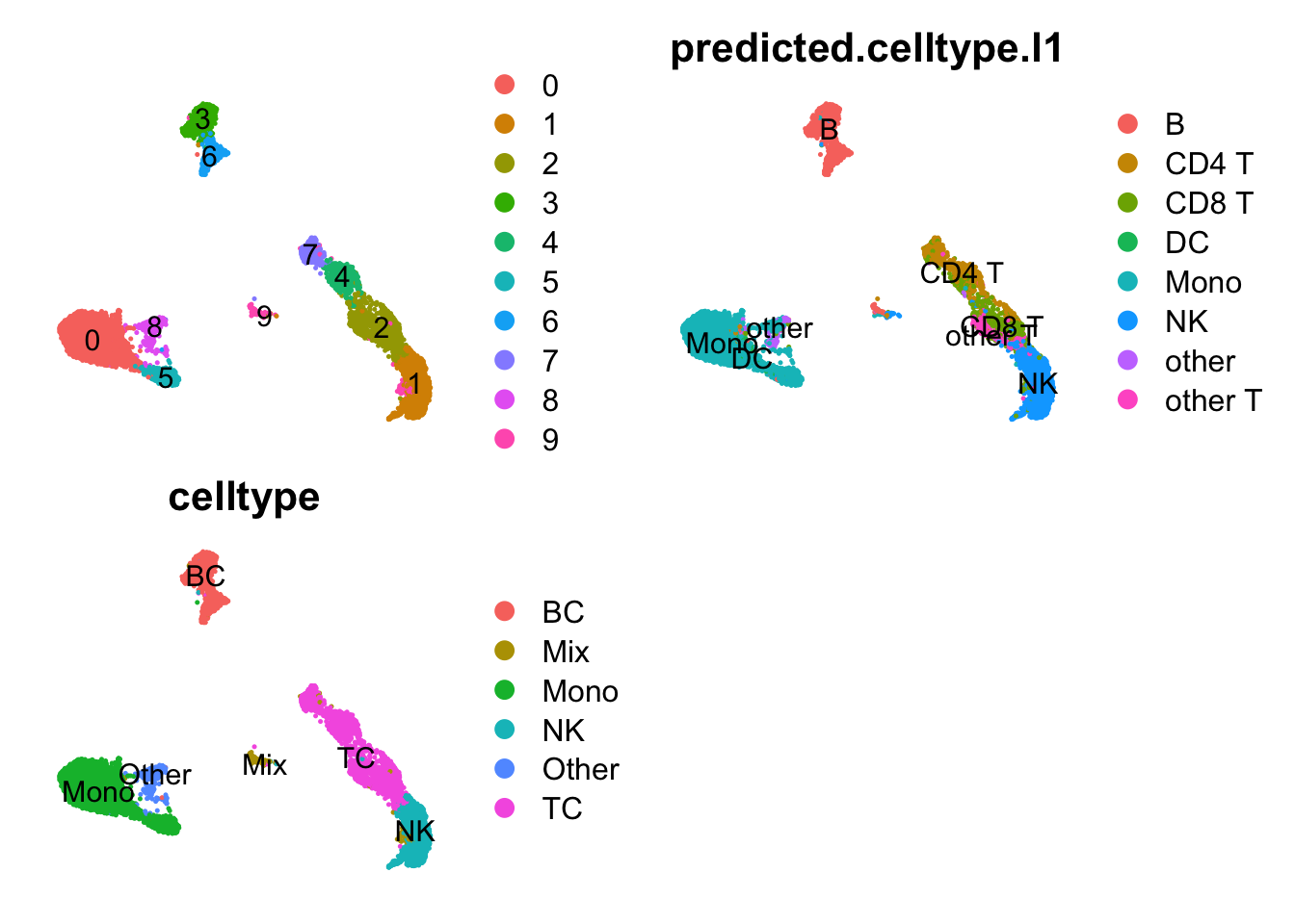
sobj = SetIdent(sobj, value = "celltype")2.3 SCT merged
Run with all cells considered a single sample.
sobj = SCTransform(sobj, new.assay.name = "SCT", verbose = F)
ndata$sct_data = sobj@assays$SCT@data
ndata$sct_counts = sobj@assays$SCT@counts

VlnPlot(sobj, c("CD3E","CD14","CCR7","RPL10"), assay = "SCT", slot = "data", ncol=4)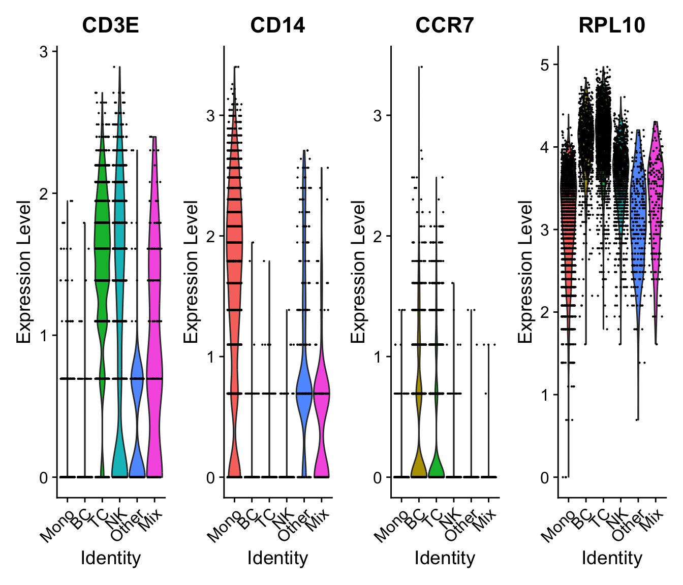
VlnPlot(sobj, c("CD3E","CD14","CCR7","RPL10"), assay = "SCTL", slot = "data", ncol=4)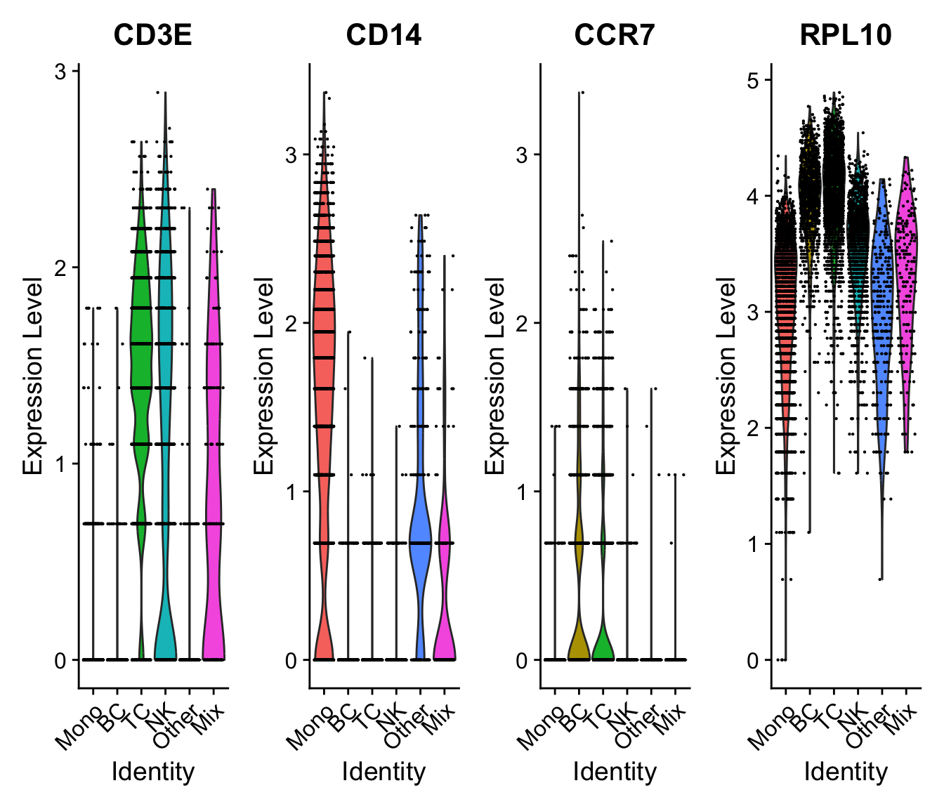
Returns a Seurat object with a new assay (named SCT by default) with counts being (corrected) counts, data being log1p(counts), scale.data being pearson residuals
dim(sobj@assays$RNA@layers$counts)[1] 17513 7134dim(sobj@assays$SCT@counts)[1] 17513 7134dim(sobj@assays$SCT@scale.data)[1] 3000 7134wrap_plots(
FeatureScatter(sobj, "nCount_RNA","nCount_SCT", group.by = "orig.ident") + NoLegend(),
FeatureScatter(sobj, "nFeature_RNA","nFeature_SCT", group.by = "orig.ident") + NoLegend(),
FeatureScatter(sobj, "nCount_RNA","nCount_SCTL", group.by = "orig.ident") + NoLegend(),
FeatureScatter(sobj, "nFeature_RNA","nFeature_SCTL", group.by = "orig.ident")+ NoLegend(),
ncol = 2
)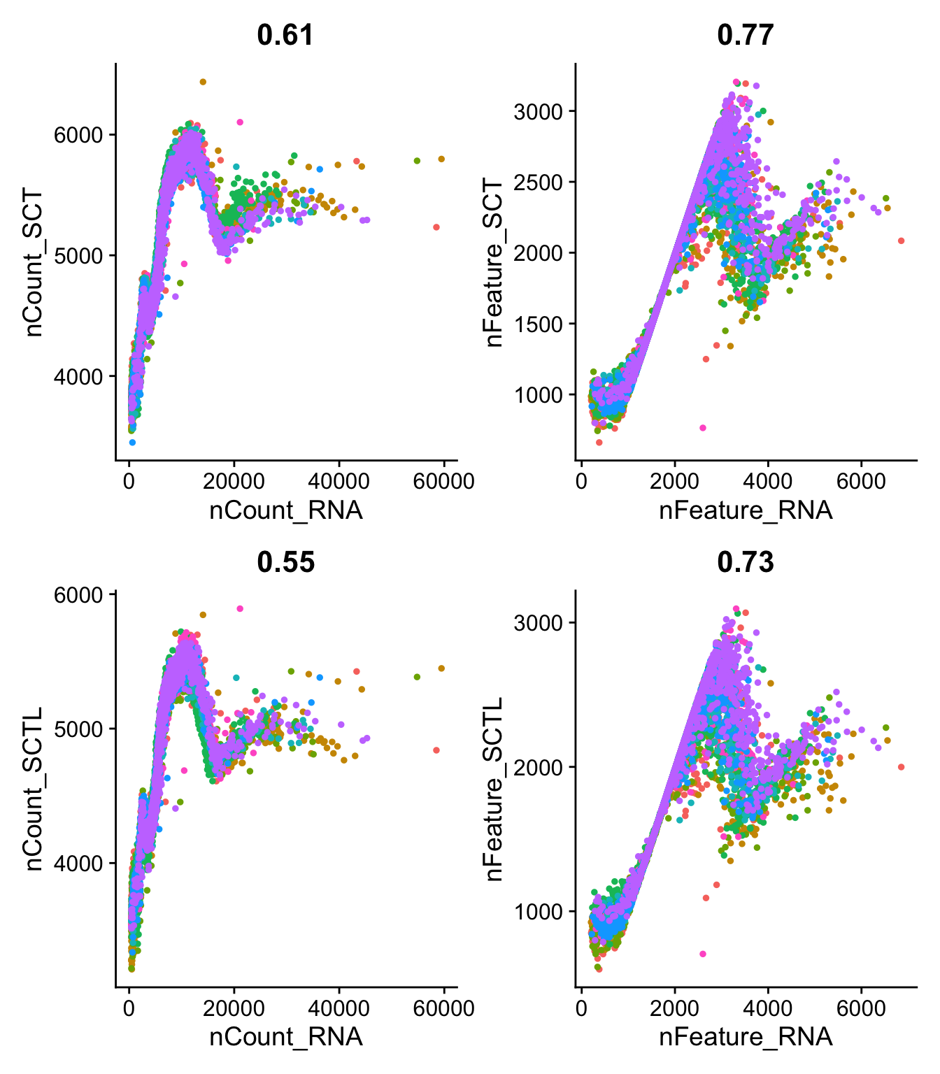
range(sobj$nFeature_RNA)[1] 201 6853range(sobj$nFeature_SCT)[1] 661 3205VlnPlot(sobj, c("nCount_RNA","nCount_SCT", "nCount_SCTL")) + NoLegend()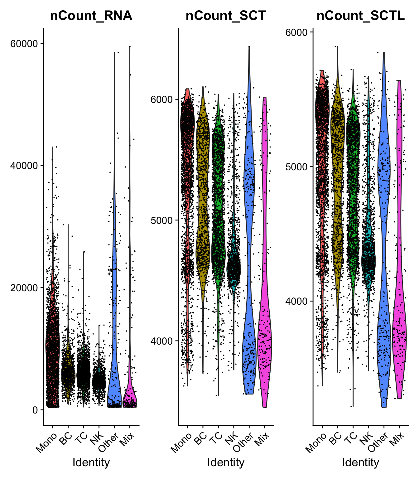
VlnPlot(sobj, c("nFeature_RNA","nFeature_SCT", "nFeature_SCTL")) + NoLegend() 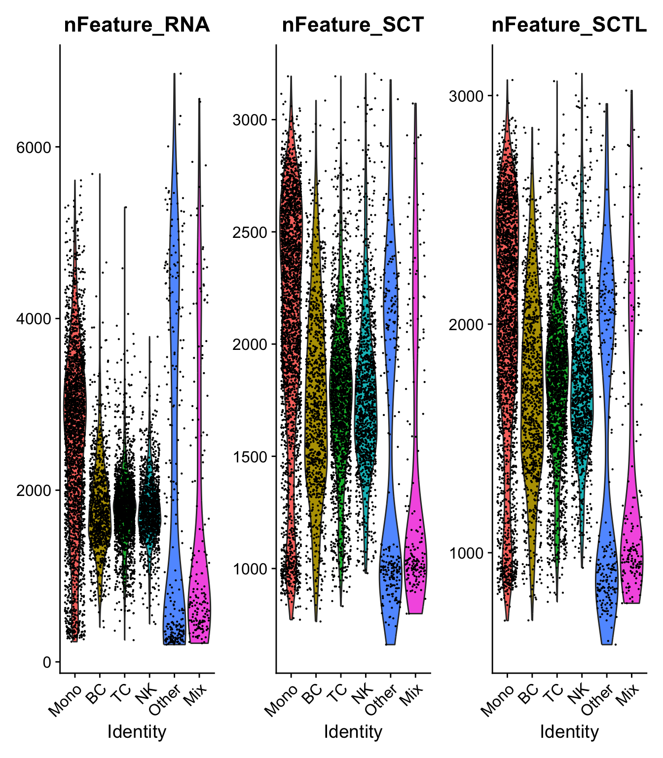
Much lower number of features per cell, especially in the high nF cells. But also higher lowest number of features. How can the nFeatures increase?
Seems like it is mainly genes that are high in most cells that get “imputed” counts in SCT, but they are still low.
Plot stats per gene:
df.genes = data.frame(
  nCell_RNA=rowSums(ndata$counts>0),
  nUMI_RNA=rowSums(ndata$counts),
  nCell_SCT=rowSums(ndata$sct_counts>0),
  nUMI_SCT=rowSums(ndata$sct_counts))

wrap_plots(
ggplot(df.genes, aes(x=nCell_RNA,y=nCell_SCT)) + geom_point() + theme_classic(),
ggplot(df.genes, aes(x=nUMI_RNA,y=nUMI_SCT)) + geom_point() + theme_classic() + scale_x_log10() + scale_y_log10(),
ggplot(df.genes, aes(x=nUMI_RNA,y=nCell_RNA)) + geom_point() + theme_classic() + scale_x_log10(),
ggplot(df.genes, aes(x=nUMI_SCT,y=nCell_SCT)) + geom_point() + theme_classic() + scale_x_log10(),
ncol = 2
)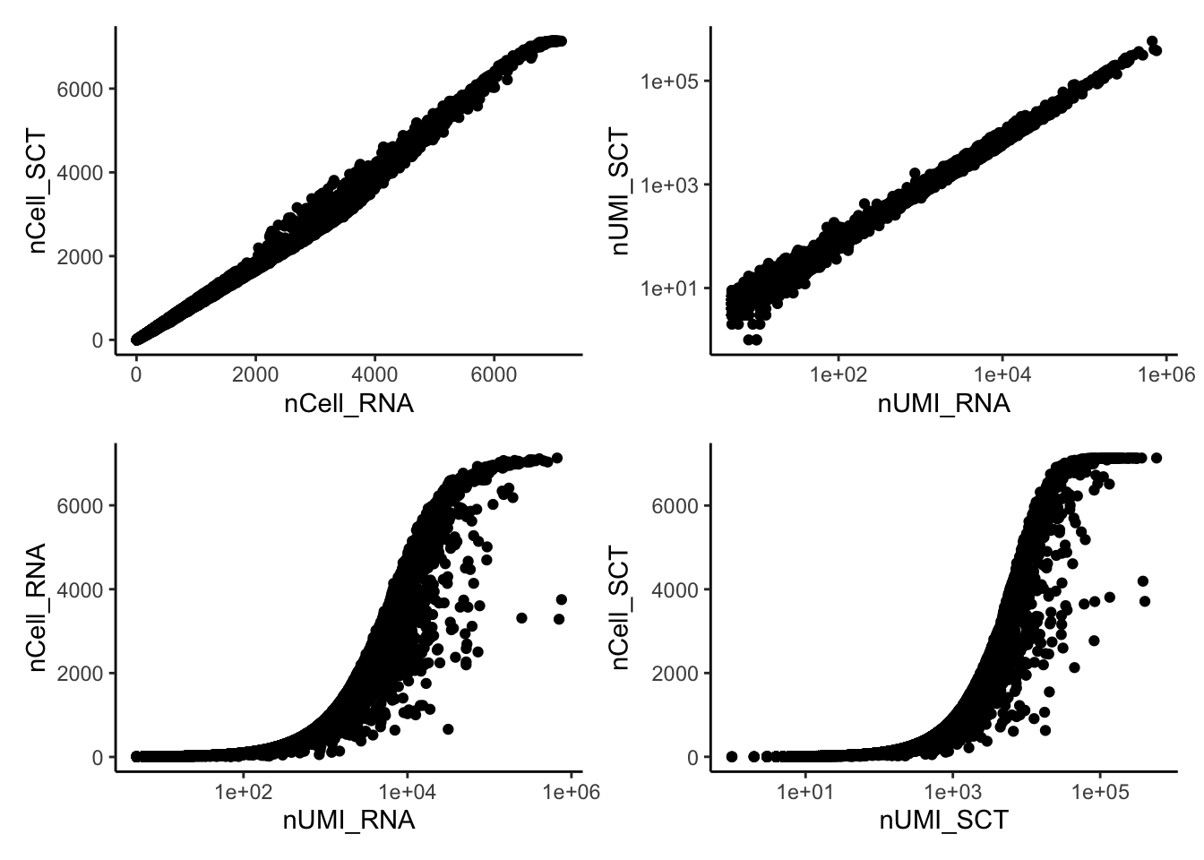
Each gene is found in a similar number of cells, but the nUMI per gene is much lower with SCT
Get residuals for all of the hvgs
sobj@active.assay = "SCT"
sobj = PrepSCTIntegration(list(s = sobj), anchor.features = intersect(rownames(sobj), hvg))$s
# some of the hvgs are not in the SCT assay!
ndata$sct_scaledata = sobj@assays$SCT@scale.data


dim(sobj@assays$SCT@scale.data)
[1] 4972 7134Many cells have counts for genes where there was no detection. Check for instance chrY genes and the XIST gene. That we know should mainly be in males/females.
genes_file <- file.path(path_seurat, "genes_table.csv")
genes.table <- read.csv(genes_file)
genes.table <- genes.table[genes.table$external_gene_name %in% rownames(sobj), ]

par1 = c(10001, 2781479)
par2 = c(56887903, 57217415)
p1.gene = genes.table$external_gene_name[genes.table$start_position > par1[1] & genes.table$start_position < par1[2] & genes.table$chromosome_name == "Y"]
p2.gene = genes.table$external_gene_name[genes.table$start_position > par2[1] & genes.table$start_position < par2[2] & genes.table$chromosome_name == "Y"]

chrY.gene <- genes.table$external_gene_name[genes.table$chromosome_name == "Y"]
chrY.gene = setdiff(chrY.gene, c(p1.gene, p2.gene))

sobj <- PercentageFeatureSet(sobj, features = chrY.gene, col.name = "pct_chrY_SCT", assay = "SCT")
# SCTL has fewer genes in the count matrix,
sobj <- PercentageFeatureSet(sobj, features = intersect(chrY.gene, rownames(sobj@assays$SCTL@counts)), col.name = "pct_chrY_SCTL", assay = "SCTL")
sobj <- PercentageFeatureSet(sobj, features = chrY.gene, col.name = "pct_chrY_RNA", assay = "RNA")


VlnPlot(sobj, group.by = "orig.ident", features = c("pct_chrY_RNA", "pct_chrY_SCT","pct_chrY_SCTL"))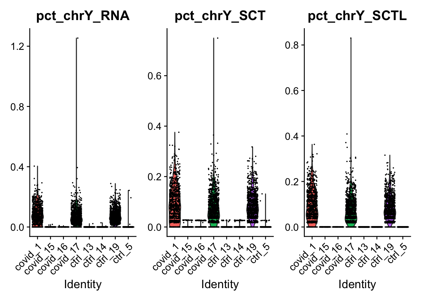
ChrY genes have low counts in the female cells with SCT. But not in SCTL which is run per sample, so SCT borrows information across the samples.
p1 = VlnPlot(sobj, group.by = "orig.ident", features = "XIST", assay = "RNA", slot = "data") + NoLegend()
p2 = VlnPlot(sobj, group.by = "orig.ident", features = "XIST", assay = "SCT", slot = "data") + NoLegend()

p3 = VlnPlot(sobj, group.by = "orig.ident", features = "XIST", assay = "SCTL", slot = "data") + NoLegend()

p1 + p2 + p3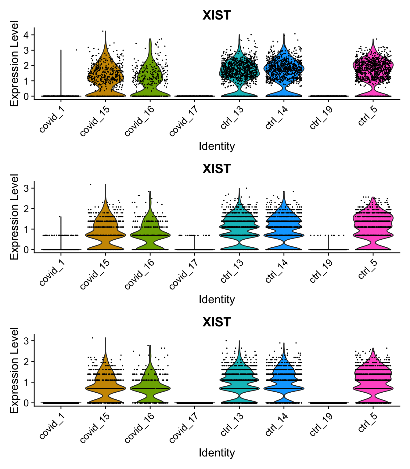
Same for XIST expression.
2.4 Subsample
From now, use a smaller dataset.
Select 10 cells per sample and cluster to make a smaller dataset for the comparison. Use resolution 1 with 11 clusters.
Then filter again for genes detected in at least 5 cells.
dim(sobj)[1] 17513 7134sobj@active.assay = "RNA"
sobj = DietSeurat(sobj, assays = "RNA")
sobj$clust_sample = paste0(sobj$RNA_snn_res.1, sobj$orig.ident)
sobj = SetIdent(sobj, value = "clust_sample")
sobj = subset(sobj, cells = WhichCells(sobj, downsample = 10))
nC = rowSums(sobj@assays$RNA@layers$counts > 0)
sobj = sobj[nC>4,]
dim(sobj)[1] 13363 928Also subset all normdata for the same cells/genes, and also the subset of variable genes
hvg = intersect(rownames(sobj),hvg)

for (n in names(ndata)){
  tmp = intersect(hvg, rownames(ndata[[n]]))
  ndata[[n]] = ndata[[n]][tmp,colnames(sobj)]
}

# clean memory
gc()
used (Mb) gc trigger (Mb) limit (Mb) max used (Mb)
Ncells 9499543 507.4 16614665 887.4 NA 16614665 887.4
Vcells 81518697 622.0 586678216 4476.0 65536 733231275 5594.22.5 Scalefactors lognorm
First plot counts and default lognorm (sf=10K) and calculate scale.data for the different normalizations.
Also calculate hvgs to get dispersions at different scale factors.
2.5.1 SF 10K
sobj = SetIdent(sobj, value =  "RNA_snn_res.0.5")

#VlnPlot(sobj, c("CD3E","CD14","CCR7","RPL10"), slot = "counts", ncol=4)
#VlnPlot(sobj, c("CD3E","CD14","CCR7","RPL10"), slot = "data", ncol=4)


# vagenes for 10k
vinfo = list()
tmp = FindVariableFeatures(sobj, selection.method = "mean.var.plot", verbose = F, assay = "RNA")
vinfo[["10k"]] = tmp@assays$RNA@meta.data


sobj = ScaleData(sobj, features = hvg, assay = "RNA")
D = sobj@assays$RNA@layers$scale.data
rownames(D) = hvg
colnames(D) = colnames(sobj)
ndata$lognorm10k_scaledata = D

cd3plots = list()
cd3plots[[1]] = VlnPlot(sobj, features = "CD3E") + NoAxes() + ggtitle("10K") + NoLegend()
2.5.2 SF 1K
tmp = NormalizeData(sobj, scale.factor = 1000, verbose = F)

tmp = FindVariableFeatures(tmp, selection.method = "mean.var.plot", verbose = F, assay = "RNA")
vinfo[["1k"]] = tmp@assays$RNA@meta.data


D = tmp@assays$RNA@layers$data
rownames(D) = rownames(sobj)
colnames(D) = colnames(sobj)
ndata$lognorm1k = D[hvg,]
#VlnPlot(tmp, c("CD3E","CD14","CCR7","RPL10"), slot = "data", ncol=4)

tmp = ScaleData(tmp, features = hvg, assay = "RNA")
D = tmp@assays$RNA@layers$scale.data
rownames(D) = hvg
colnames(D) = colnames(sobj)
ndata$lognorm1k_scaledata = D

cd3plots[[2]] = VlnPlot(tmp, features = "CD3E") + NoAxes() + ggtitle("1K") + NoLegend()
2.5.3 SF 100K
tmp = NormalizeData(sobj, scale.factor = 100000, verbose = F)

D = tmp@assays$RNA@layers$data
rownames(D) = rownames(sobj)
colnames(D) = colnames(sobj)
ndata$lognorm100k = D[hvg,]

tmp = ScaleData(tmp, features = hvg, assay = "RNA")
D = tmp@assays$RNA@layers$scale.data
rownames(D) = hvg
colnames(D) = colnames(sobj)
ndata$lognorm100k_scaledata = D

tmp = FindVariableFeatures(tmp, selection.method = "mean.var.plot", verbose = F, assay = "RNA")
vinfo[["100k"]] = tmp@assays$RNA@meta.data

#VlnPlot(tmp, c("CD3E","CD14","CCR7","RPL10"), slot = "data", ncol=4)

cd3plots[[3]] = VlnPlot(tmp, features = "CD3E") + NoAxes() + ggtitle("100K") + NoLegend()
wrap_plots(cd3plots, ncol = 3)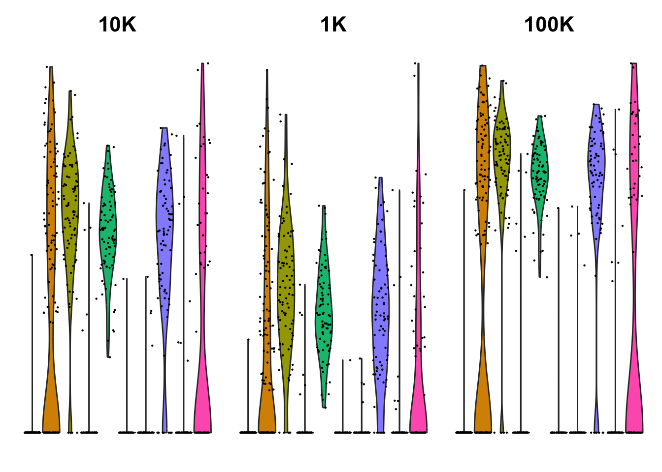
Clearly gives a larger difference to zero with larger size factors. So the dispersion will be higher.
In principle is the same as changing the pseudocount which is now 1.
2.5.4 Dispersions
Plot the estimated dispersions with mvp vs mean.
vinfo = vinfo[sort(names(vinfo))]

plots = list()
for (n in names(vinfo)){
  plots[[n]] = ggplot(vinfo[[n]], aes(x=vf_mvp_data_mvp.mean, y=vf_mvp_data_mvp.dispersion.scaled, color = vf_mvp_data_variable)) + geom_point()+ ggtitle(paste0(n, " - ", sum(vinfo[[n]]$vf_mvp_data_variable), " hvgs")) + theme_classic() + NoLegend()
}

wrap_plots(plots, ncol=2)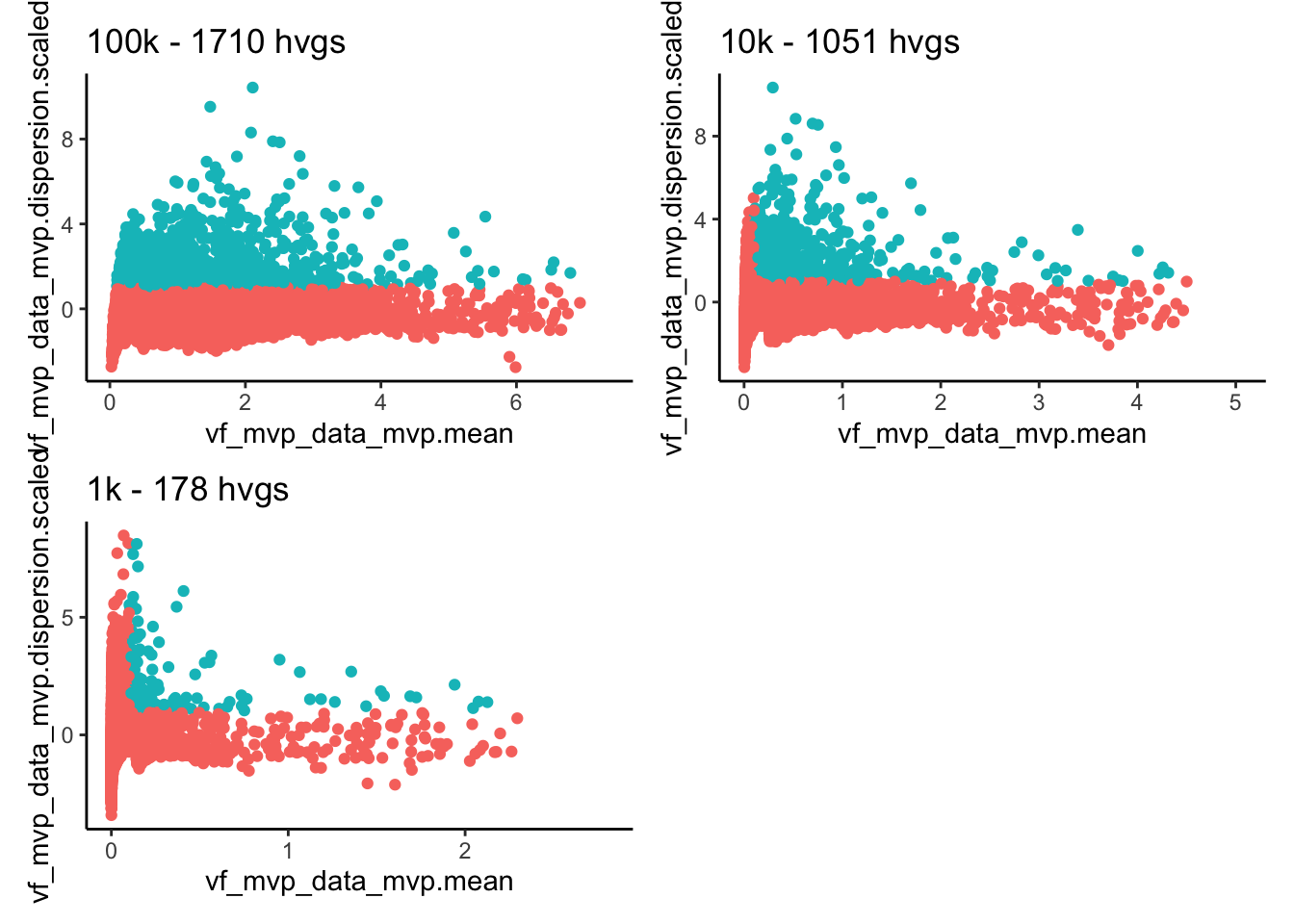
Much higher dispersions and more variable genes with 100K, very low with 1k.
The cutoffs are dispersions over 1 and mean 0.1-8
disp = data.frame(Reduce(cbind,lapply(vinfo, function(x) x$vf_mvp_data_mvp.dispersion.scaled)))
colnames(disp) = names(vinfo)
plot(disp)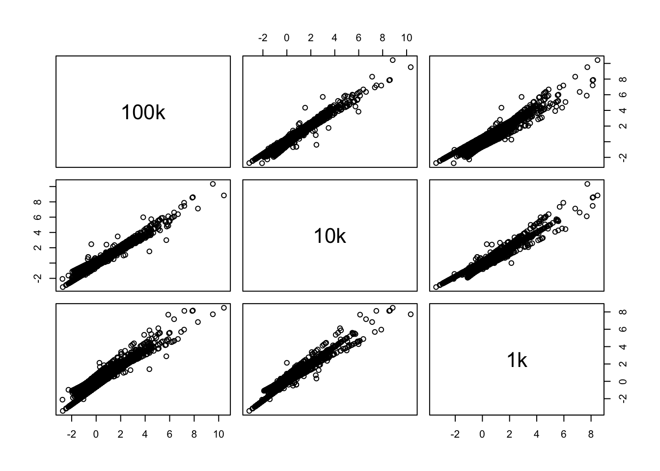
Still similar trend on the dispersions, the same genes have high dispersion.
2.6 Logcounts
Log of counts without depth normalization
ndata$logcounts = log1p(ndata$counts)2.7 TMM
Run EdgeR TMM,
# TMM
dge = edgeR::DGEList(sobj@assays$RNA@layers$counts)
dge <- edgeR::normLibSizes(dge, method = "TMM")
tmp  = edgeR::cpm(dge) # is with log = FALSE
colnames(tmp) = colnames(sobj)
tmp = tmp[rownames(sobj) %in% hvg,]
rownames(tmp) = hvg
ndata$tmm = tmp

tmp = edgeR::cpm(dge, log = TRUE)
colnames(tmp) = colnames(sobj)
tmp = tmp[rownames(sobj) %in% hvg,]
rownames(tmp) = hvg
ndata$tmm_log = tmp
2.8 Quantile
limma-voom quantile
# should be run on the lognorm values. use the full dataset to calculate.
tmp = limma::voom(sobj@assays$RNA@layers$data,normalize.method = "quantile")$E
colnames(tmp) = colnames(sobj)
rownames(tmp) = rownames(sobj)
ndata$quantile = tmp[hvg,]
2.9 Deconvolution
Run quickCluster and then computeSumFactors.
library(scran)
set.seed(100)

sce = as.SingleCellExperiment(sobj)
cl = quickCluster(sce)
table(cl)
cl
1 2 3 4 5 6
172 157 159 186 126 128 sce <- computeSumFactors(sce, cluster=cl, min.mean=0.1)
sce <- logNormCounts(sce)
assayNames(sce)[1] "counts" "logcounts"tmp = assay(sce, "logcounts")
tmp = tmp[hvg,]
ndata$deconv = tmp2.10 Pearson residuals
Using the method implemented in scanpy.
penv = "/Users/asabjor/miniconda3/envs/scanpy_2024_nopip"
norm.scanpy = basiliskRun(env=penv, fun=function(counts) {
    scanpy <- reticulate::import("scanpy")
    ad = reticulate::import("anndata")
    adata = ad$AnnData(counts)
    print(adata$X[1:10,1:10])
    #sc.experimental.pp.normalize_pearson_residuals(adata)
    scanpy$experimental$pp$normalize_pearson_residuals(adata)
    return(list(norm=adata$X))

}, counts = t(sobj@assays$RNA@layers$counts),  testload="scanpy")
10 x 10 sparse Matrix of class "dgCMatrix"
[1,] . . . . . . . . . .
[2,] . . . . . . . . . .
[3,] . . . . . . . . . .
[4,] . . . 3 . . . 2 . .
[5,] . . . . . . 1 . . .
[6,] . . . . . . . . . .
[7,] . . . . . . . 1 . .
[8,] . . . . . . . . . .
[9,] . . . 1 . . . . . .
[10,] . . 1 . . . . . . .rownames(norm.scanpy$norm) = colnames(sobj)
colnames(norm.scanpy$norm) = rownames(sobj)
ndata$pearson = t(norm.scanpy$norm[,hvg])2.11 CD3 violins
Plot cd3 violins for these different normalizations.
cd3 = data.frame(Reduce(cbind, lapply(ndata, function(x) x["CD3E",])))
colnames(cd3)=names(ndata)
cd3$clusters = sobj@active.ident

df = reshape2::melt(cd3, id = "clusters")
df$variable = factor(df$variable, levels = sort(names(ndata)))

ggplot(df, aes(x=clusters, y=value, fill=clusters)) + geom_violin(trim = T, scale = "width" , adjust = 1) + facet_wrap(~variable, scales = "free")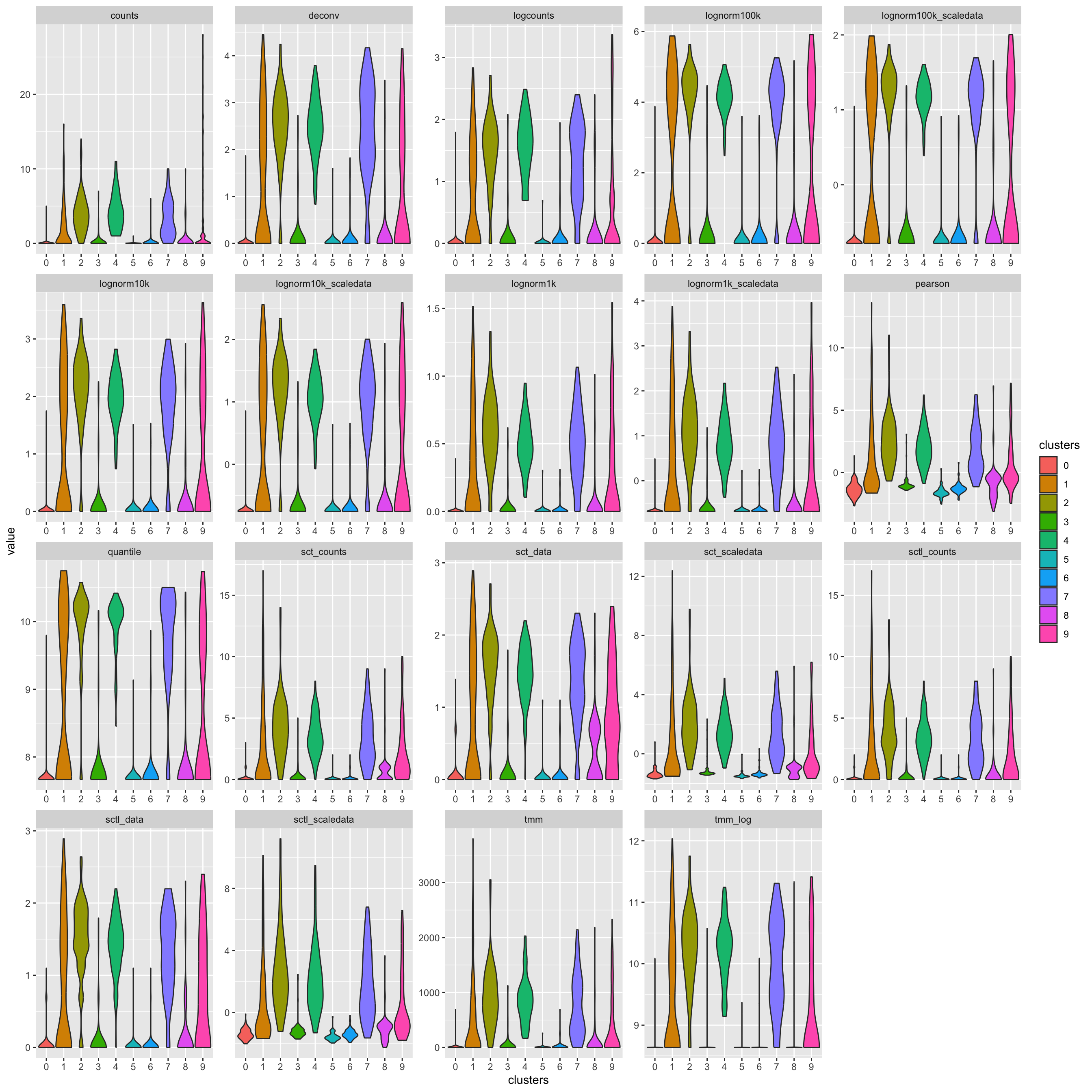
3 Distributions
Plot the expression distribution for a few single cells using each method. Select cells with highest/medium/lowest total counts.
cs = colSums(ndata$counts)
r = order(cs)
sel = r[c(1,460,length(r))]
cs[sel]
covid_1_TTGTGTTAGACATAAC-1 covid_1_CGCATGGTCGATACAC-1
90 1226
covid_15_CACGAATAGAAGCCAC-15
20443 subset = lapply(ndata, function(x) x[,sel])
plots = list()
for (ds in sort(names(subset))){
l = reshape2::melt(data.frame(subset[[ds]]))
plots[[ds]] = ggplot(l, aes(x=value)) + geom_histogram(bins = 200) + theme_classic() + facet_wrap(~variable, scales="free") + scale_y_log10() + ggtitle(ds)
}
wrap_plots(plots[1:6], ncol=1)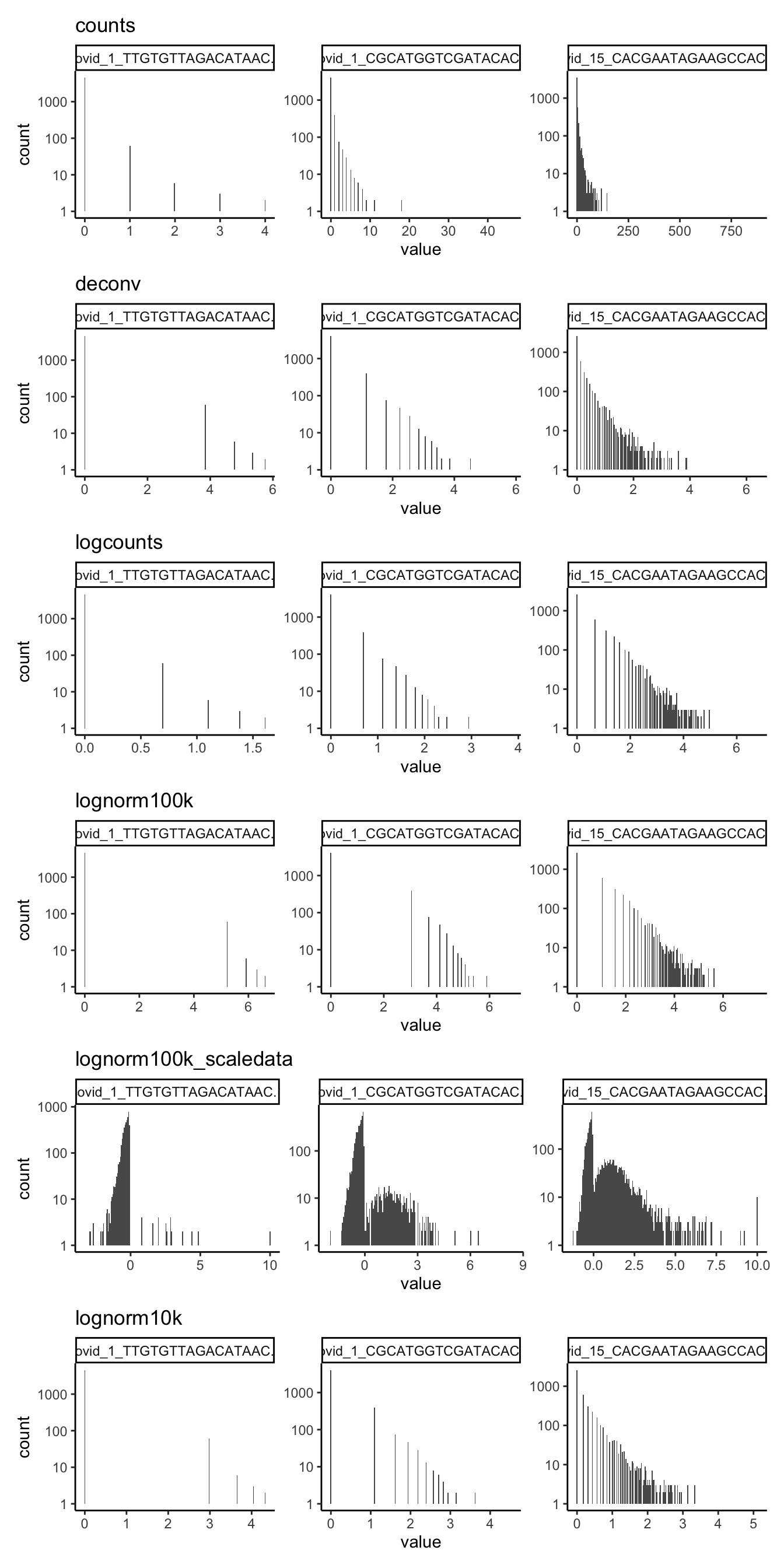
wrap_plots(plots[7:12], ncol=1)
wrap_plots(plots[13:length(plots)], ncol=1)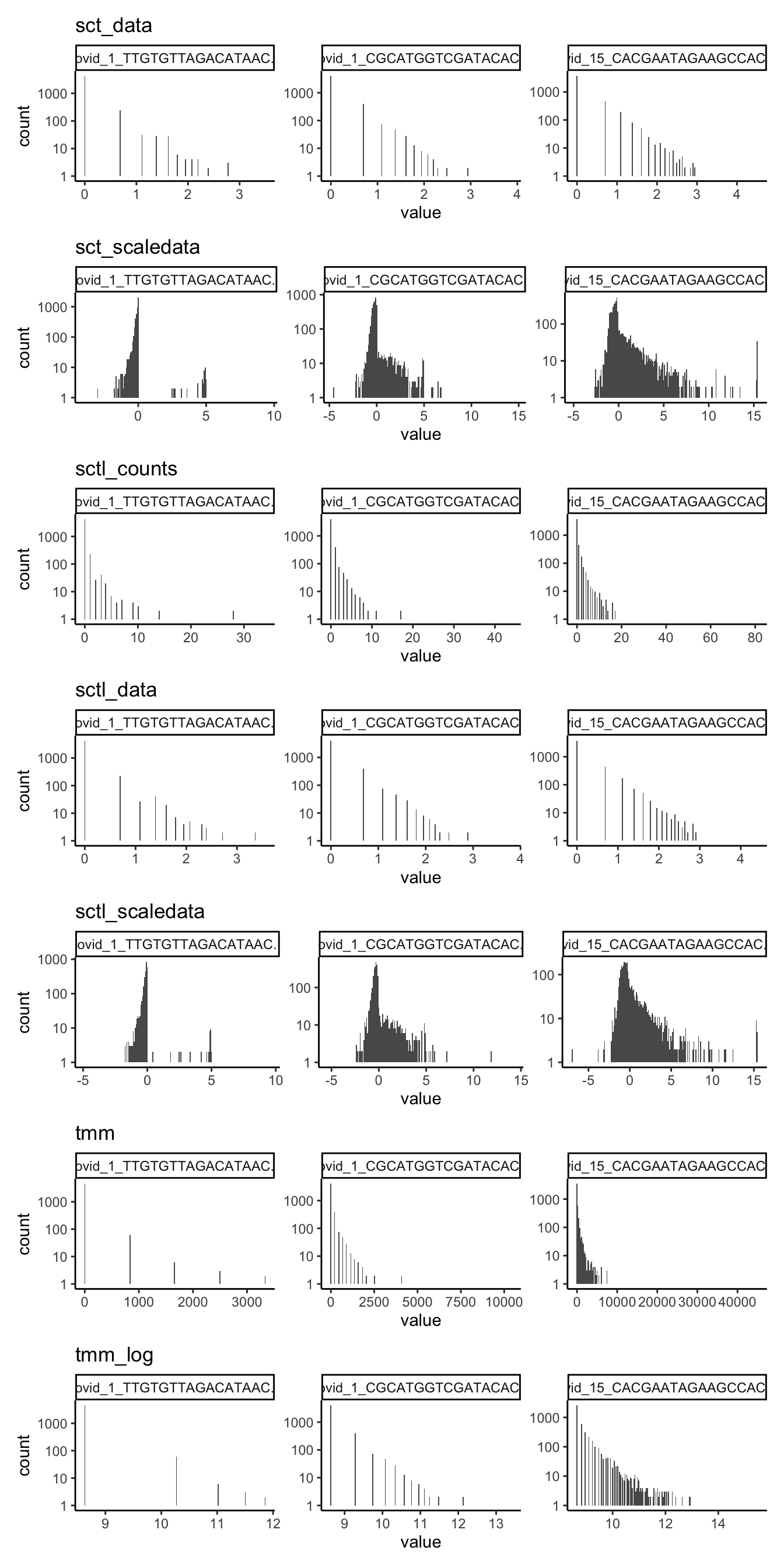
4 Cell correlations
For all the different normalizations, calculate the correlation between cells. For a fair comparison, use the same set of genes.
Except for the scaledata for SCTL that has too few genes!
# corSparse function copied from Signac package utilities.R

corSparse <- function(X, Y = NULL, cov = FALSE) {
  X <- as(object = X, Class = "CsparseMatrix")
  n <- nrow(x = X)
  muX <- colMeans(x = X)

  if (!is.null(x = Y)) {
    if (nrow(x = X) != nrow(x = Y)) {
      stop("Matrices must contain the same number of rows")
    }
    Y <- as(object = Y, Class = "CsparseMatrix")
    muY <- colMeans(x = Y)
    covmat <- ( as.matrix(x = crossprod(x = X, y = Y)) - n * tcrossprod(x = muX, y = muY) ) / (n-1)
    sdvecX <- sqrt( (colSums(x = X^2) - n*muX^2) / (n-1) )
    sdvecY <- sqrt( (colSums(x = Y^2) - n*muY^2) / (n-1) )
    cormat <- covmat / tcrossprod(x = sdvecX, y = sdvecY)
  } else {
    covmat <- ( as.matrix(crossprod(x = X)) - n * tcrossprod(x = muX) ) / (n-1)
    sdvec <- sqrt(x = diag(x = covmat))
    cormat <- covmat / tcrossprod(x = sdvec)
  }
  if (cov) {
    dimnames(x = covmat) <- NULL
    return(covmat)
  } else {
    dimnames(x = cormat) <- NULL
    return(cormat)
  }
}
# have fewer genes for sctl-scaledata, still use the same set for all other samples ignoring that sctl has fewer!
t = table(unlist(lapply(ndata, rownames)))
selG = names(t)[t >= (length(ndata)-1)]
ndata = lapply(ndata, function(x) x[intersect(rownames(x),selG),])
cors = list()
for (n in sort(names(ndata))){
print(n)
cors[[n]] = corSparse(ndata[[n]])
}[1] "counts"
[1] "deconv"
[1] "logcounts"
[1] "lognorm100k"
[1] "lognorm100k_scaledata"
[1] "lognorm10k"
[1] "lognorm10k_scaledata"
[1] "lognorm1k"
[1] "lognorm1k_scaledata"
[1] "pearson"
[1] "quantile"
[1] "sct_counts"
[1] "sct_data"
[1] "sct_scaledata"
[1] "sctl_counts"
[1] "sctl_data"
[1] "sctl_scaledata"
[1] "tmm"
[1] "tmm_log"#cors = lapply(ndata, function(x) corSparse(x))breaks = seq(-0.5,1,0.01)
cc = lapply(cors, function(x)
hist(x[upper.tri(x)],breaks=breaks,plot=F)$counts)
count.hist = data.frame(Reduce(cbind,cc))
colnames(count.hist) = names(ndata)
count.hist$breaks = breaks[-1]
c = Reduce(cbind, lapply(cors, function(x) x[upper.tri(x)]))
colnames(c) = names(cors)
long = reshape2::melt(c)
ggplot(long, aes(x=value)) + geom_histogram(bins=100) +
facet_wrap(~Var2, scales = "free_y") + geom_vline(xintercept =0, color="red") 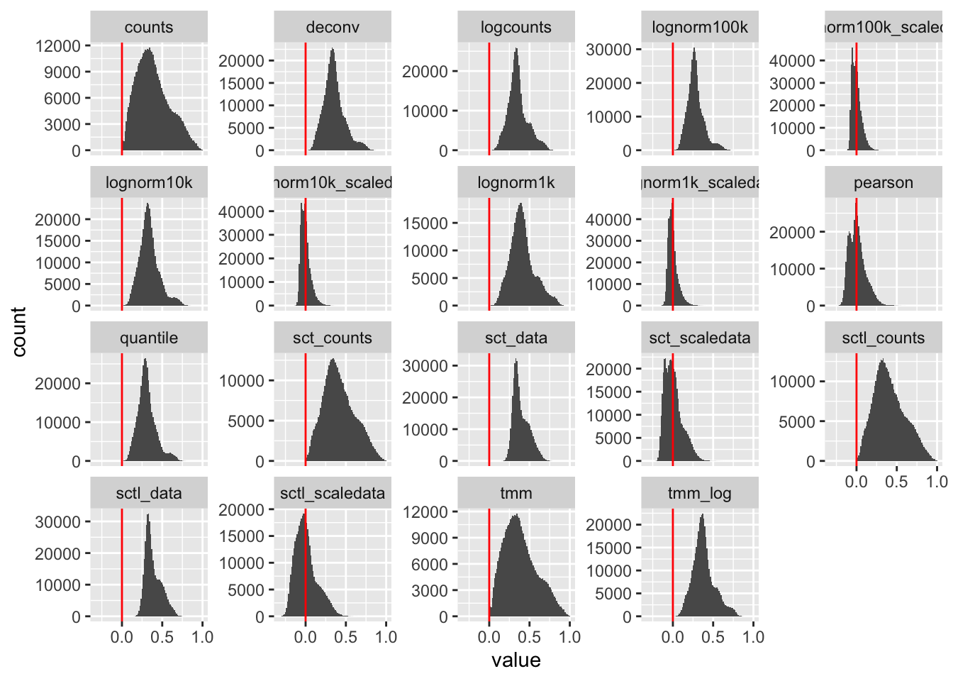
stats = apply(c, 2, summary)
t(stats)
Min. 1st Qu. Median Mean
counts -5.088535e-03 0.23230169 0.359057137 0.3876623832
deconv 8.952432e-04 0.26950424 0.339649442 0.3531730611
logcounts 7.587383e-04 0.27896786 0.341350609 0.3563585870
lognorm100k -1.893007e-04 0.21737202 0.269881348 0.2823120771
lognorm100k_scaledata -1.358677e-01 -0.04628789 -0.009354206 -0.0006189914
lognorm10k 5.124563e-04 0.25871941 0.326215623 0.3391142020
lognorm10k_scaledata -1.526215e-01 -0.04516235 -0.010395184 -0.0008814526
lognorm1k 9.819781e-04 0.31014511 0.394088563 0.4114224291
lognorm1k_scaledata -1.701344e-01 -0.04335472 -0.011190967 -0.0008133232
pearson -2.726683e-01 -0.06906390 -0.003071477 0.0081909333
quantile 1.156027e-03 0.23670468 0.296213401 0.3091003740
sct_counts 5.518484e-03 0.27753797 0.393958830 0.4186517500
sct_data 1.465805e-01 0.32142427 0.368884265 0.3945946018
sct_scaledata -2.323186e-01 -0.07915305 -0.010833788 0.0067053275
sctl_counts 4.692851e-03 0.26913139 0.385389128 0.4121448393
sctl_data 1.394500e-01 0.31327415 0.359751049 0.3863770802
sctl_scaledata -3.169345e-01 -0.09450794 -0.015246042 0.0047925770
tmm -5.088535e-03 0.23230169 0.359057137 0.3876623832
tmm_log -1.111245e-05 0.29547126 0.367618514 0.3826587382
3rd Qu. Max.
counts 0.51888427 0.9979323
deconv 0.41745624 0.8869059
logcounts 0.41555708 0.8166209
lognorm100k 0.33086334 0.7858652
lognorm100k_scaledata 0.03124555 0.6449176
lognorm10k 0.40025879 0.8698278
lognorm10k_scaledata 0.02789470 0.6953211
lognorm1k 0.49042499 0.9429184
lognorm1k_scaledata 0.02594518 0.7124583
pearson 0.06466442 0.6892138
quantile 0.36465779 0.8355153
sct_counts 0.54749577 0.9975654
sct_data 0.46084588 0.7892639
sct_scaledata 0.06634267 0.7227993
sctl_counts 0.54059869 0.9971110
sctl_data 0.45209032 0.8058592
sctl_scaledata 0.07696892 0.7767212
tmm 0.51888427 0.9979323
tmm_log 0.44942367 0.88487545 Clustering
Run a quick umap/clustering with the different normalizations. All with same set of genes, pca with 20 PCs,
# need to run the commands to get all setting correct in the seurat object.
sobj.all =  CreateSeuratObject(counts = ndata$counts[selG,])
sobj.all = NormalizeData(sobj.all, verbose = F)
sobj.all = ScaleData(sobj.all, verbose = F)
sobj.all$old_clust = sobj$RNA_snn_res.0.5
sobj.all$sample = sobj$orig.ident

# then run per dataset
for (ds in sort(names(ndata))){
  if (ds == "sctl_scaledata") { next }
  d = as(ndata[[ds]][selG,], "matrix")
  sobj.all@assays$RNA@layers$scale.data = d
  sobj.all = sobj.all %>% RunPCA(npcs=50,verbose = F, features = selG) %>% RunUMAP(dims=1:20, verbose = F) %>% FindNeighbors(dims=1:20, verbose = F) %>% FindClusters(resolution = 0.6, verbose = F)
  sobj.all[[paste0("umap_",ds)]] = sobj.all[["umap"]]
  sobj.all[[paste0("clusters_",ds)]] = sobj.all[["seurat_clusters"]]
  sobj.all[[paste0("pca_",ds)]] = sobj.all[["pca"]]
}
Gene detection in all:
plots = list()
for (ds in sort(names(ndata))){
  if (ds == "sctl_scaledata") { next }
  plots[[ds]] = FeaturePlot(sobj.all, features = "nFeature_RNA", reduction = paste0("umap_",ds), pt.size = .2) + NoLegend() + NoAxes() + ggtitle(ds) + theme(plot.title = element_text(size = 6))
}

wrap_plots(plots, ncol=4)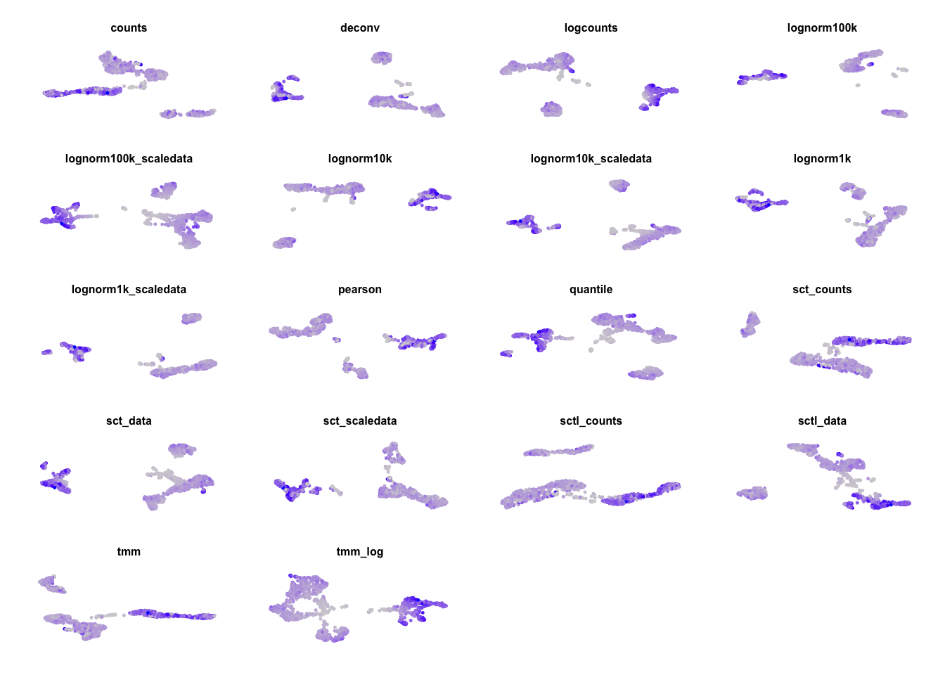
Celltype predictions in all:
plots = list()
sobj.all$celltype = sobj[,colnames(sobj.all)]$celltype

for (ds in sort(names(ndata))){
  if (ds == "sctl_scaledata") { next }
  plots[[ds]] = DimPlot(sobj.all, group.by = "celltype", label = T, label.size = 2, reduction = paste0("umap_",ds), pt.size = .2) + NoLegend() + NoAxes() + ggtitle(ds) + theme(plot.title = element_text(size = 6))
}

wrap_plots(plots, ncol=4)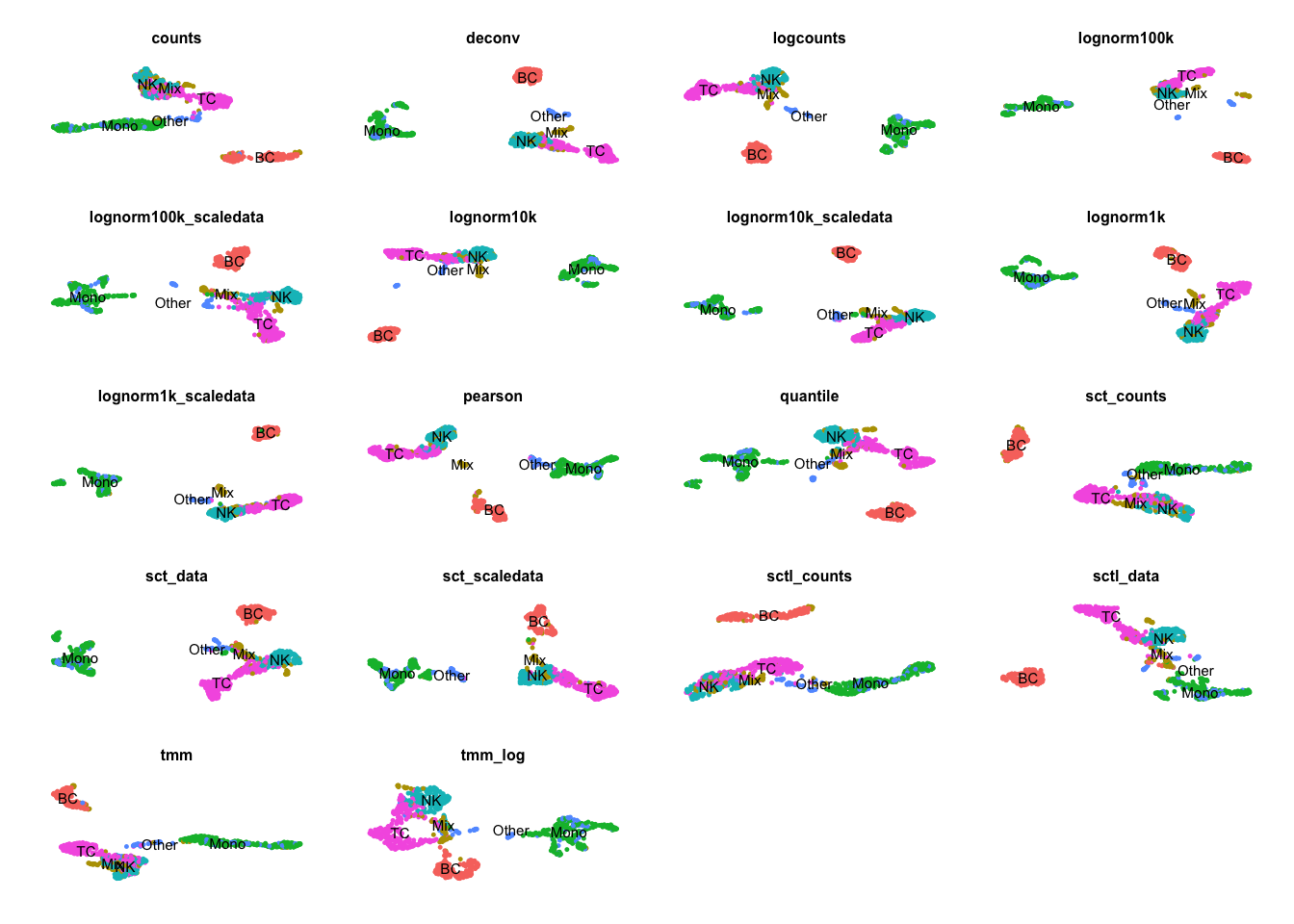
5.0.1 PCs stats
5.0.1.1 Contribution to variance
How much variance is in each pc, among the 50 PCs calculated. Plot for first 10 PCs
nplot = 10

pcs = names(sobj.all@reductions)[grepl("pca_", names(sobj.all@reductions))]

std = lapply(pcs, function(x) Stdev(sobj.all, reduction = x))

variance_explained <- data.frame(Reduce(cbind,lapply(std, function(x) (x^2 / sum(x^2) * 100)[1:nplot])))
colnames(variance_explained) = pcs

variance_explained$PC = factor(as.character(1:nrow(variance_explained)), levels = as.character(1:nrow(variance_explained)))
df = reshape2::melt(variance_explained[1:10,])

ggplot(df, aes(x=PC, y=value)) + geom_bar(stat="identity") + facet_wrap(~variable)
For TMM and quantile, pretty much all variance is in PC1.
More flat for the scaled data and for residuals.
Also more flat with lower size factors.
5.0.1.2 PC correlation to different stats
Correlation to nFeatures - plot as R-squared.
emb = lapply(pcs, function(x) Embeddings(sobj.all, reduction = x))

plot_pc_correl = function(emb, feature){
  f = as.matrix(sobj[[feature]])
  cors = Reduce(rbind,lapply(emb, function(x) {
      apply(x[,1:10],2,function(y) summary(lm(y ~ f))$r.squared)
    }))

  df = data.frame(t(cors))
  colnames(df) = pcs
  df$PC = factor(as.character(1:10), levels = as.character(1:10))

  df2 = reshape2::melt(df)
  df2$value = abs(df2$value)

  ggplot(df2, aes(x=PC, y=value)) + geom_bar(stat="identity") + facet_wrap(~variable)
}

plot_pc_correl(emb, "nFeature_RNA")
Most methods have PC1 dominated by nFeatures, but more so for logcounts, lognorm with large size factors and bulk methods.
Same for mito genes and total counts:
plot_pc_correl(emb, "percent_mito")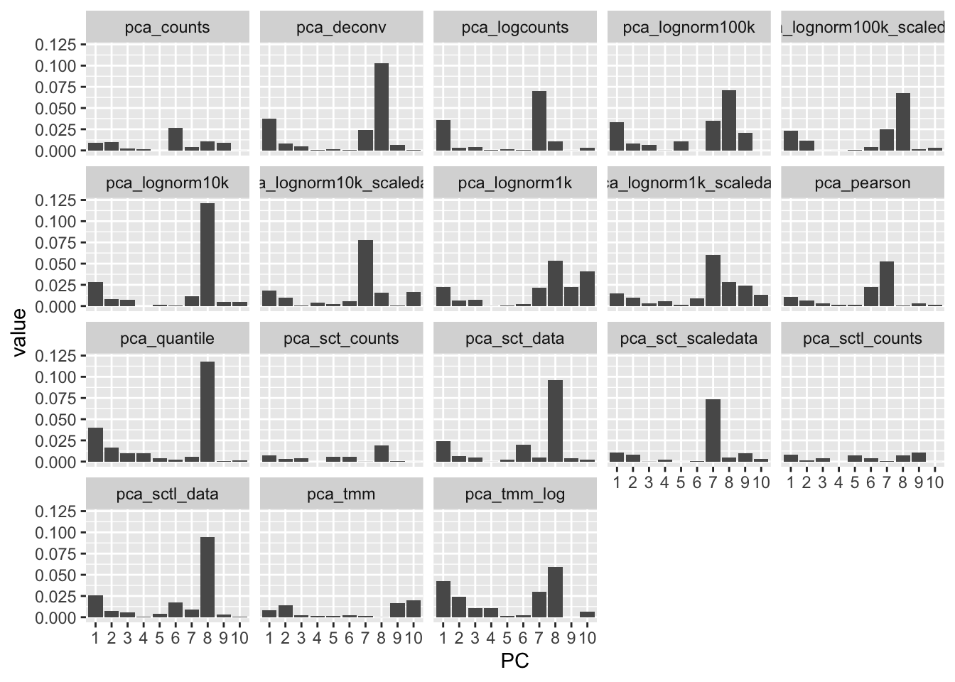
plot_pc_correl(emb, "nCount_RNA")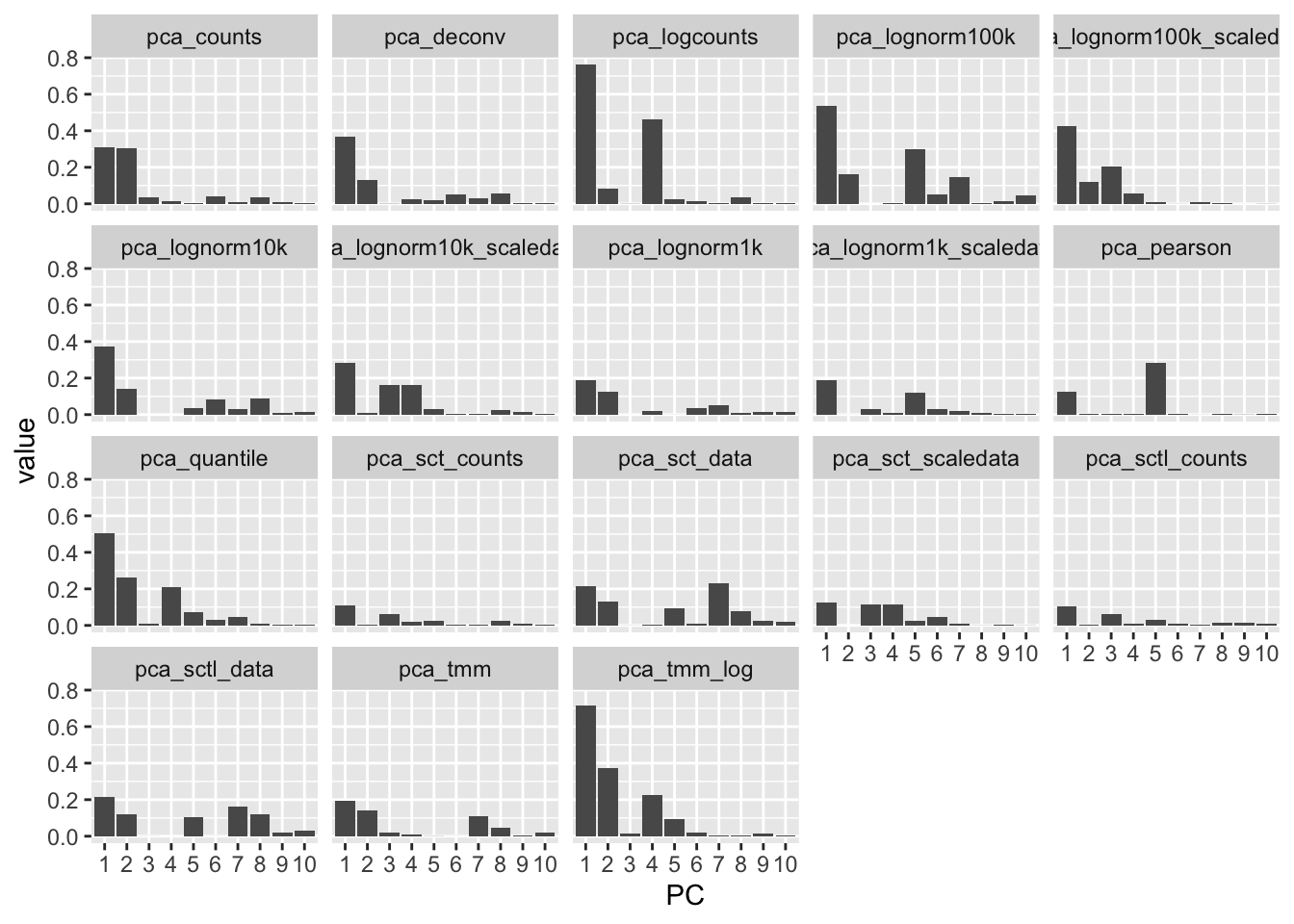
Vs celltypes:
plot_pc_correl(emb, "celltype")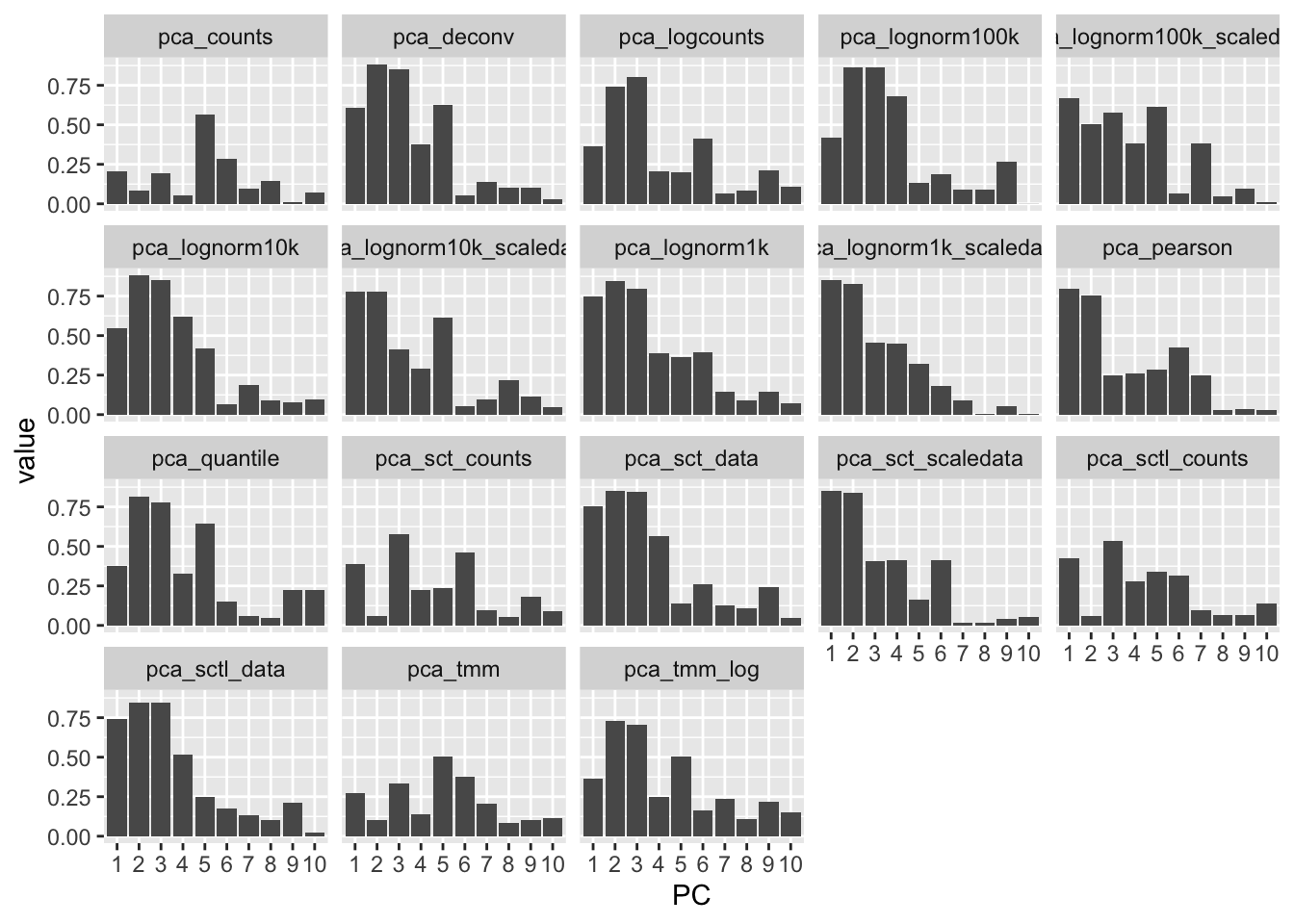
6 DGE
Run DGE detection between 2 clusters, do NK vs T-cell, using the differently normalized data and compare results.
One parametric test (MAST), one rank-based (wilcoxon). Select 150 cells of each celltype.
Just for lognorm, deconvolution, sct data, tmm-log and logcounts.
# select 150 cells from each celltype
sobj = SetIdent(sobj, value = "celltype")
selC = intersect(colnames(sobj)[which(sobj$celltype %in% c("NK","TC"))], WhichCells(sobj, downsample = 150))
tmp = sobj[selG,selC]


# then run per dataset
markersM = list()
sel.methods = c("lognorm10k","deconv","logcounts","sct_data","tmm_log")

for (ds in sel.methods){
  d = as(ndata[[ds]][rownames(tmp),selC], "matrix")
  tmp@assays$RNA@layers$data = d
  markersM[[paste0("M-",ds)]] = FindMarkers(tmp, ident.1 = "TC", ident.2 = "NK", test.use = "MAST")
  markersM[[paste0("W-",ds)]] = FindMarkers(tmp, ident.1 = "TC", ident.2 = "NK", test.use = "wilcox")
}
Select significant genes below 0.01. OBS! test only among 4.6K genes, so adjusted pvalue is lower than it should.
signM = lapply(markersM, function(x) {
  up = rownames(x)[x$avg_log2FC>0 & x$p_val_adj < 0.01]
  down = rownames(x)[x$avg_log2FC<0 & x$p_val_adj < 0.01]
  return(list(up=up, down=down))
})

nM = Reduce(cbind, lapply(signM, function(x)  c(length(x$up), length(x$down))))
colnames(nM) = names(signM)
rownames(nM) = c("TC","NK")

df = reshape2::melt(nM)
ggplot(df, aes(x=Var2, y=value, fill = Var1)) + geom_bar(stat = "identity") + theme_classic() + RotatedAxis() + ggtitle("Number of significant genes") 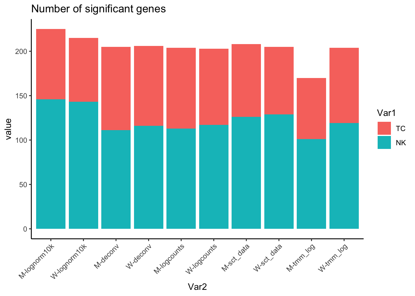
Select all genes enriched in NK, top 100 genes
l1 = lapply(signM, function(x) x$down[1:100])


o = overlap_phyper2(l1,l1, silent = T,  remove.diag = T)
m = o$M[1:length(l1), 1:length(l1)]
diag(m) = NA
pheatmap(m, display_numbers = m, main="top 100 NK genes")
Same for Tcell degs, fewer significant genes, take top 65
l1 = lapply(signM, function(x) x$up[1:65])


o = overlap_phyper2(l1,l1, silent = T,  remove.diag = T)
m = o$M[1:length(l1), 1:length(l1)]
diag(m) = NA
pheatmap(m, display_numbers = m, main="top 65 TC genes")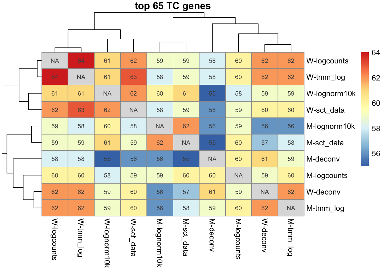
For TC genes 55 - 64 genes overlap among top 65. For NK genes 90 - 99 of top 100 genes overlap.
Quite similar regardless of normalization.
7 Session info
Click here
sessionInfo()R version 4.3.3 (2024-02-29)
Platform: x86_64-apple-darwin13.4.0 (64-bit)
Running under: macOS Big Sur ... 10.16
Matrix products: default
BLAS/LAPACK: /Users/asabjor/miniconda3/envs/seurat5_u/lib/libopenblasp-r0.3.28.dylib; LAPACK version 3.12.0
locale:
[1] sv_SE.UTF-8/sv_SE.UTF-8/sv_SE.UTF-8/C/sv_SE.UTF-8/sv_SE.UTF-8
time zone: Europe/Stockholm
tzcode source: system (macOS)
attached base packages:
[1] stats4 stats graphics grDevices utils datasets methods
[8] base
other attached packages:
[1] pheatmap_1.0.12 dplyr_1.1.4
[3] basilisk_1.14.1 scran_1.30.0
[5] scuttle_1.12.0 SingleCellExperiment_1.24.0
[7] SummarizedExperiment_1.32.0 Biobase_2.62.0
[9] GenomicRanges_1.54.1 GenomeInfoDb_1.38.1
[11] IRanges_2.36.0 S4Vectors_0.40.2
[13] BiocGenerics_0.48.1 MatrixGenerics_1.14.0
[15] matrixStats_1.5.0 patchwork_1.3.0
[17] ggplot2_3.5.1 Matrix_1.6-5
[19] Seurat_5.1.0 SeuratObject_5.0.2
[21] sp_2.1-4
loaded via a namespace (and not attached):
[1] RcppAnnoy_0.0.22 splines_4.3.3
[3] later_1.4.1 bitops_1.0-9
[5] filelock_1.0.3 tibble_3.2.1
[7] polyclip_1.10-7 basilisk.utils_1.14.1
[9] fastDummies_1.7.4 lifecycle_1.0.4
[11] edgeR_4.0.16 globals_0.16.3
[13] lattice_0.22-6 MASS_7.3-60.0.1
[15] MAST_1.28.0 magrittr_2.0.3
[17] limma_3.58.1 plotly_4.10.4
[19] rmarkdown_2.29 remotes_2.5.0
[21] yaml_2.3.10 metapod_1.10.0
[23] httpuv_1.6.15 glmGamPoi_1.14.0
[25] sctransform_0.4.1 spam_2.11-0
[27] sessioninfo_1.2.2 pkgbuild_1.4.5
[29] spatstat.sparse_3.1-0 reticulate_1.40.0
[31] cowplot_1.1.3 pbapply_1.7-2
[33] RColorBrewer_1.1-3 pkgload_1.4.0
[35] abind_1.4-5 zlibbioc_1.48.0
[37] Rtsne_0.17 presto_1.0.0
[39] purrr_1.0.2 RCurl_1.98-1.16
[41] GenomeInfoDbData_1.2.11 ggrepel_0.9.6
[43] irlba_2.3.5.1 listenv_0.9.1
[45] spatstat.utils_3.1-2 goftest_1.2-3
[47] RSpectra_0.16-2 spatstat.random_3.3-2
[49] dqrng_0.3.2 fitdistrplus_1.2-2
[51] parallelly_1.41.0 DelayedMatrixStats_1.24.0
[53] leiden_0.4.3.1 codetools_0.2-20
[55] DelayedArray_0.28.0 tidyselect_1.2.1
[57] farver_2.1.2 ScaledMatrix_1.10.0
[59] spatstat.explore_3.3-4 jsonlite_1.8.9
[61] BiocNeighbors_1.20.0 ellipsis_0.3.2
[63] progressr_0.15.1 ggridges_0.5.6
[65] survival_3.8-3 progress_1.2.3
[67] tools_4.3.3 ica_1.0-3
[69] Rcpp_1.0.13-1 glue_1.8.0
[71] gridExtra_2.3 SparseArray_1.2.2
[73] xfun_0.50 usethis_3.1.0
[75] withr_3.0.2 fastmap_1.2.0
[77] bluster_1.12.0 digest_0.6.37
[79] rsvd_1.0.5 R6_2.5.1
[81] mime_0.12 colorspace_2.1-1
[83] scattermore_1.2 tensor_1.5
[85] spatstat.data_3.1-4 tidyr_1.3.1
[87] generics_0.1.3 data.table_1.15.4
[89] prettyunits_1.2.0 httr_1.4.7
[91] htmlwidgets_1.6.4 S4Arrays_1.2.0
[93] uwot_0.1.16 pkgconfig_2.0.3
[95] gtable_0.3.6 lmtest_0.9-40
[97] XVector_0.42.0 htmltools_0.5.8.1
[99] profvis_0.4.0 dotCall64_1.2
[101] scales_1.3.0 png_0.1-8
[103] spatstat.univar_3.1-1 knitr_1.49
[105] reshape2_1.4.4 curl_6.0.1
[107] nlme_3.1-165 cachem_1.1.0
[109] zoo_1.8-12 stringr_1.5.1
[111] KernSmooth_2.23-26 vipor_0.4.7
[113] parallel_4.3.3 miniUI_0.1.1.1
[115] ggrastr_1.0.2 pillar_1.10.1
[117] grid_4.3.3 vctrs_0.6.5
[119] RANN_2.6.2 urlchecker_1.0.1
[121] promises_1.3.2 BiocSingular_1.18.0
[123] beachmat_2.18.0 xtable_1.8-4
[125] cluster_2.1.8 beeswarm_0.4.0
[127] evaluate_1.0.1 cli_3.6.3
[129] locfit_1.5-9.10 compiler_4.3.3
[131] rlang_1.1.4 crayon_1.5.3
[133] future.apply_1.11.2 labeling_0.4.3
[135] ggbeeswarm_0.7.2 fs_1.6.5
[137] plyr_1.8.9 stringi_1.8.4
[139] viridisLite_0.4.2 deldir_2.0-4
[141] BiocParallel_1.36.0 munsell_0.5.1
[143] lazyeval_0.2.2 devtools_2.4.5
[145] spatstat.geom_3.3-4 dir.expiry_1.10.0
[147] RcppHNSW_0.6.0 hms_1.1.3
[149] sparseMatrixStats_1.14.0 future_1.34.0
[151] statmod_1.5.0 shiny_1.10.0
[153] ROCR_1.0-11 memoise_2.0.1
[155] igraph_2.0.3