suppressPackageStartupMessages({
    library(Seurat)
    library(zellkonverter)
    library(Matrix)
    library(ggplot2)
    library(patchwork)
    library(scran)
    library(ComplexHeatmap)
    library(basilisk)
})

devtools::source_url("https://raw.githubusercontent.com/asabjorklund/single_cell_R_scripts/main/overlap_phyper_v2.R")With data in place, now we can start loading libraries we will use in this tutorial.
1 Load data
OBS! Zellkonverter installs conda env with basilisk! Takes a while to run first time!!
path_results <- "data/covid/results"
if (!dir.exists(path_results)) dir.create(path_results, recursive = T)
path_seurat = "../seurat/data/covid/results/"
path_bioc = "../bioc/data/covid/results/"
path_scanpy = "../scanpy/data/covid/results/"
path_results <- "data/covid/results"
if (!dir.exists(path_results)) dir.create(path_results, recursive = T)
path_seurat = "../seurat/data/covid/results/"
path_bioc = "../bioc/data/covid/results/"
path_scanpy = "../scanpy/data/covid/results/"
# fetch the files with qc and dimred for each
# seurat
sobj = readRDS(file.path(path_seurat,"seurat_covid_qc_dr_int_cl.rds"))
# bioc
sce = readRDS(file.path(path_bioc,"bioc_covid_qc_dr_int_cl.rds"))
bioc = as.Seurat(sce)
# scanpy
scanpy.sce = readH5AD(file.path(path_scanpy, "scanpy_covid_qc_dr_scanorama_cl.h5ad"))
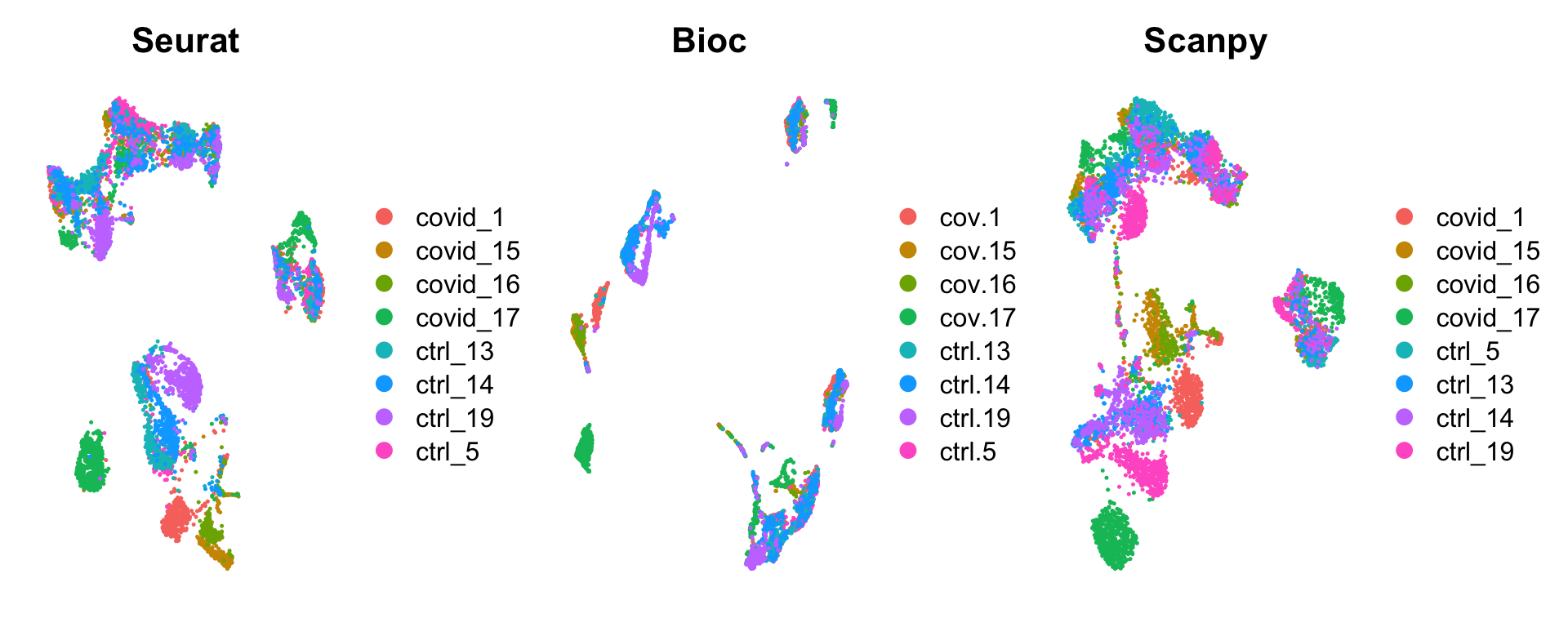
scanpy = as.Seurat(scanpy.sce, counts = NULL, data = "X") # only have the var.genes data that is scaled.2 Umaps
wrap_plots(
    DimPlot(sobj, group.by = "orig.ident") + NoAxes() + ggtitle("Seurat"),
    DimPlot(bioc, group.by = "sample") + NoAxes() + ggtitle("Bioc"),
    DimPlot(scanpy, group.by = "sample", reduction = "X_umap_uncorr") + NoAxes() + ggtitle("Scanpy"),
    ncol = 3
)
Create one dataset with the cells that are present in all samples. Also add in umap from all 3 pipelines.
meta.seurat = sobj@meta.data
meta.scanpy = scanpy@meta.data
meta.bioc = bioc@meta.data

meta.bioc$cell = rownames(meta.bioc)
meta.scanpy$cell = sapply(rownames(meta.scanpy), function(x) substr(x,1,nchar(x)-2))
meta.seurat$cell = unlist(lapply(strsplit(rownames(meta.seurat),"_"), function(x) x[3]))
in.all = intersect(intersect(meta.scanpy$cell, meta.seurat$cell), meta.bioc$cell)
tmp1 = meta.bioc[match(in.all, meta.bioc$cell),]
colnames(tmp1) = paste0(colnames(tmp1),"_bioc")
tmp2 = meta.scanpy[match(in.all, meta.scanpy$cell),]
colnames(tmp2) = paste0(colnames(tmp2),"_scpy")
all = sobj[,match(in.all, meta.seurat$cell)]
meta.all = cbind(all@meta.data, tmp1,tmp2)
all@meta.data = meta.all
Reductions(all) [1] "pca" "umap" "tsne"
[4] "UMAP10_on_PCA" "UMAP_on_ScaleData" "integrated_cca"
[7] "umap_cca" "tsne_cca" "harmony"
[10] "umap_harmony" "scanorama" "scanoramaC"
[13] "umap_scanorama" "umap_scanoramaC" tmp = bioc@reductions$UMAP_on_PCA@cell.embeddings[match(in.all, meta.bioc$cell),]
rownames(tmp) = colnames(all)
all[["umap_bioc"]] = CreateDimReducObject(tmp, key = "umapbioc_", assay = "RNA")
tmp = scanpy@reductions$X_umap_uncorr@cell.embeddings[match(in.all, meta.scanpy$cell),]
rownames(tmp) = colnames(all)
all[["umap_scpy"]] = CreateDimReducObject(tmp, key = "umapscpy_", assay = "RNA")
Reductions(all) [1] "pca" "umap" "tsne"
[4] "UMAP10_on_PCA" "UMAP_on_ScaleData" "integrated_cca"
[7] "umap_cca" "tsne_cca" "harmony"
[10] "umap_harmony" "scanorama" "scanoramaC"
[13] "umap_scanorama" "umap_scanoramaC" "umap_bioc"
[16] "umap_scpy" 3 Variable features
In Seurat, FindVariableFeatures is not batch aware unless the data is split into layers by samples, here we have the variable genes created with layers. In Bioc modelGeneVar we used sample as a blocking parameter, e.g calculates the variable genes per sample and combines the variances. Similar in scanpy we used the samples as batch_key.
hvgs = list()
hvgs$seurat = VariableFeatures(sobj)
hvgs$bioc = sce@metadata$hvgs
# scanpy has no strict number on selection, instead uses dispersion cutoff. So select instead top 2000 dispersion genes.
scpy.hvg = rowData(scanpy.sce)
hvgs_scanpy = rownames(scpy.hvg)[scpy.hvg$highly_variable]
hvgs$scanpy = rownames(scpy.hvg)[order(scpy.hvg$dispersions_norm, decreasing = T)][1:2000]

cmat = make_comb_mat(hvgs)
print(cmat)
A combination matrix with 3 sets and 7 combinations.
ranges of combination set size: c(245, 869).
mode for the combination size: distinct.
sets are on rows.
Combination sets are:
seurat bioc scanpy code size
x x x 111 607
x x 110 279
x x 101 245
x x 011 344
x 100 869
x 010 770
x 001 804
Sets are:
set size
seurat 2000
bioc 2000
scanpy 2000UpSet(cmat)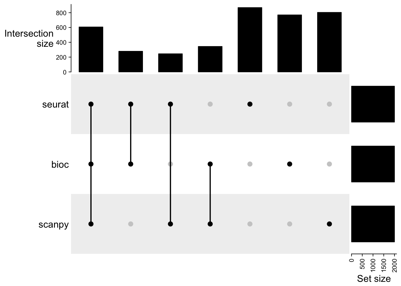
Surprisingly low overlap between the methods and many genes that are unique to one pipeline. With discrepancies in the doublet filtering the cells used differ to some extent, but otherwise the variation should be similar. Even if it is estimated in different ways.
Is the differences more due to the combination of ranks/dispersions or also found within a single dataset?
Only Seurat have the dispersions for each individual dataset stored in the object.
3.1 Compare dispersions
Recalculate for bioc.
var.out <- modelGeneVar(sce, block = sce$sample)
hvgs_bioc <- getTopHVGs(var.out, n = 2000)
cutoff <- rownames(var.out) %in% hvgs_bioc
# Merge all hvg info
all.genes = intersect(rownames(var.out), rownames(scpy.hvg))
scpy.hvg = rowData(scanpy.sce)
colnames(scpy.hvg) = paste0(colnames(scpy.hvg), "_scpy")
colnames(var.out) = paste0(colnames(var.out), "_bioc")
seu.hvg = HVFInfo(all)
all.hvg = cbind(seu.hvg[all.genes,], scpy.hvg[all.genes,], var.out[all.genes,])
par(mfrow=c(2,2))
plot(all.hvg$means_scpy, all.hvg$dispersions_norm_scpy, main = "Scanpy",pch = 16, cex = 0.4)
points(all.hvg$means_scpy[all.hvg$highly_variable_scpy], all.hvg$dispersions_norm_scpy[all.hvg$highly_variable_scpy], col="red",pch = 16, cex = 0.4)
plot(all.hvg$mean_bioc, all.hvg$bio_bioc, pch = 16, cex = 0.4, main = "Bioc")
points(all.hvg$mean_bioc[rownames(all.hvg) %in% hvgs$bioc], all.hvg$bio_bioc[rownames(all.hvg) %in% hvgs$bioc], col = "red", pch = 16, cex = .6)
plot(log1p(all.hvg$mean), all.hvg$variance.standardized, main = "Seurat",pch = 16, cex = 0.4)
points(log1p(all.hvg$mean)[match(hvgs$seurat, rownames(all.hvg))], all.hvg$variance.standardized[match(hvgs$seurat, rownames(all.hvg))],col="red",pch = 16, cex = 0.4) 
Scanpy uses min_disp=0.5, min_mean=0.0125, max_mean=3, so the highly expressed ones are not included.
Seurat uses variance.standardized to rank the genes. Bioc uses the bio slot with estimated biological variation.
all.hvg$mean_log = log1p(all.hvg$mean)
sel.means = c("mean","mean_log","means_scpy", "mean_bioc")
pairs(all.hvg[,sel.means])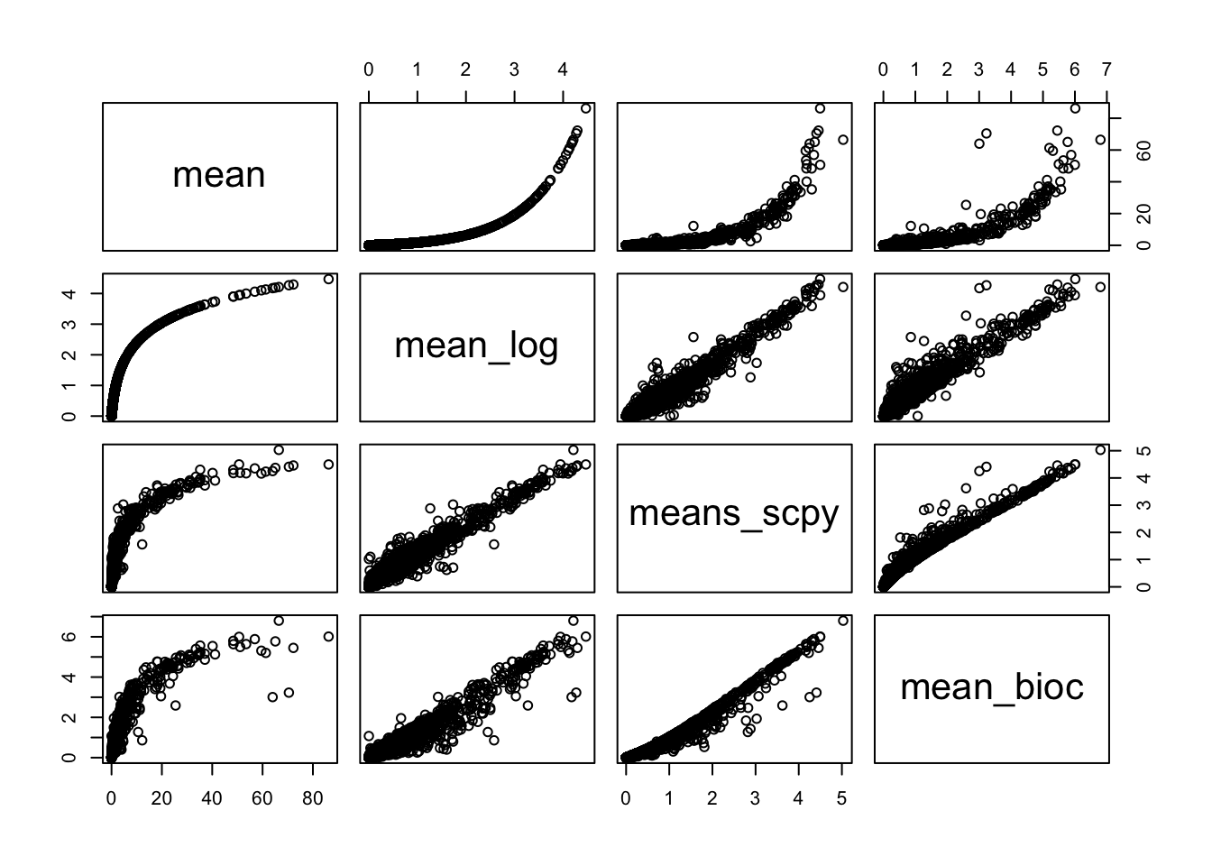
sel.disp = c("variance.standardized","dispersions_norm_scpy", "bio_bioc","total_bioc")
pairs(all.hvg[,sel.disp])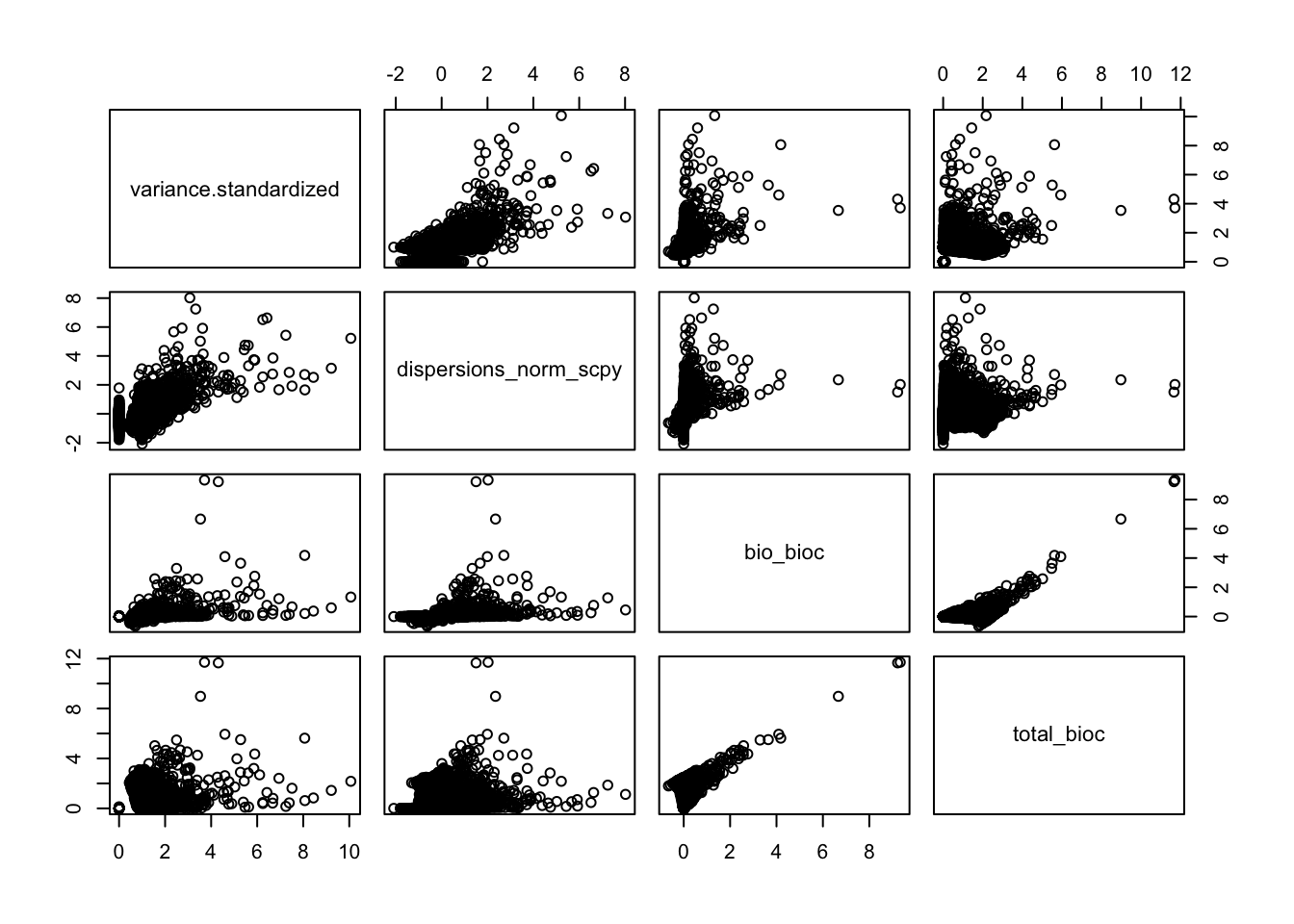
Difference in what cells were used, and also in how the dispersions across the samples is combined into one value. Do for just one sample instead.
4 For one sample
Run hvg selection for ctrl.13 sample, so that the handling of batches is not influencing results. Use default settings in all the different methods.
4.1 Seurat
Try the different methods implemented in Seurat. From the help section:
* “vst”: First, fits a line to the relationship of log(variance) and log(mean) using local polynomial regression (loess). Then standardizes the feature values using the observed mean and expected variance (given by the fitted line). Feature variance is then calculated on the standardized values after clipping to a maximum (see clip.max parameter).
* “mean.var.plot” (mvp): First, uses a function to calculate average expression (mean.function) and dispersion (dispersion.function) for each feature. Next, divides features into num.bin (deafult 20) bins based on their average expression, and calculates z-scores for dispersion within each bin. The purpose of this is to identify variable features while controlling for the strong relationship between variability and average expression
* “dispersion” (disp): selects the genes with the highest dispersion values
Feature selection for individual datasets
In each dataset, we next aimed to identify a subset of features (e.g., genes) exhibiting high variability across cells, and therefore represent heterogeneous features to prioritize for downstream analysis. Choosing genes solely based on their log-normalized single-cell variance fails to account for the mean-variance relationship that is inherent to single-cell RNA-seq. Therefore, we first applied a variance-stabilizing transformation to correct for this [Mayer et al., 2018, Hafemeister and Satija, 2019]. To learn the mean-variance relationship from the data, we computed the mean and variance of each gene using the unnormalized data (i.e., UMI or counts matrix), and applied -transformation to both. We then fit a curve to predict the variance of each gene as a function of its mean, by calculating a local fitting of polynomials of degree 2 (R function loess, span = 0.3). This global fit provided us with a regularized estimator of variance given the mean of a feature. As such, we could use it to standardize feature counts without removing higher-than-expected variation.
ctrl = all[,all$orig.ident == "ctrl_13"]
ctrl@assays$RNA@meta.data[,1:ncol(ctrl@assays$RNA@meta.data)] = NULL

ctrl = FindVariableFeatures(ctrl)
hvg_seu = list()
hvg_seu$vst = VariableFeatures(ctrl)
#top20 <- head(hvg_seu$vst, 20)
#LabelPoints(plot = VariableFeaturePlot(ctrl), points = top20, repel = TRUE)


ctrl = FindVariableFeatures(ctrl, selection.method = "mean.var.plot")
hvg_seu$mvp = VariableFeatures(ctrl)
#top20 <- head(hvg_seu$mvp, 20)
#LabelPoints(plot = VariableFeaturePlot(ctrl), points = top20, repel = TRUE)

ctrl = FindVariableFeatures(ctrl, selection.method = "dispersion")
hvg_seu$disp = VariableFeatures(ctrl)
#top20 <- head(hvg_seu$disp, 20)
#LabelPoints(plot = VariableFeaturePlot(ctrl), points = top20, repel = TRUE)

cmat = make_comb_mat(hvg_seu)
cmat
A combination matrix with 3 sets and 7 combinations.
ranges of combination set size: c(31, 1295).
mode for the combination size: distinct.
sets are on rows.
Combination sets are:
vst mvp disp code size
x x x 111 401
x x 110 31
x x 101 273
x x 011 549
x 100 1295
x 010 149
x 001 777
Sets are:
set size
vst 2000
mvp 1130
disp 2000Very little overlap between the methods in Seurat. Mvp and disp are calculated on data, while vst is done on counts.
vinfo.seu = ctrl@assays$RNA@meta.data
rownames(vinfo.seu) = rownames(ctrl)

vinfo.seu$vg_vst = rownames(vinfo.seu) %in% hvg_seu$vst
vinfo.seu$vg_disp = rownames(vinfo.seu) %in% hvg_seu$disp
vinfo.seu$vg_mvp = rownames(vinfo.seu) %in% hvg_seu$mvp
vinfo.seu$vg_vst_disp = vinfo.seu$vg_vst + vinfo.seu$vg_disp == 2
vinfo.seu$hvinfo = ifelse(vinfo.seu$vg_vst, "VST",NA)
vinfo.seu$hvinfo[vinfo.seu$vg_mvp] = "MVP"
vinfo.seu$hvinfo[vinfo.seu$vg_disp] = "DISP"
vinfo.seu$hvinfo[vinfo.seu$vg_vst_disp] = "VST/DISP"


means = colnames(vinfo.seu)[grepl("mean", colnames(vinfo.seu))]
disp = c("vf_vst_counts.ctrl_13_variance.standardized","vf_disp_data.ctrl_13_mvp.dispersion.scaled","vf_mvp_data.ctrl_13_mvp.dispersion.scaled")
pairs(vinfo.seu[,means])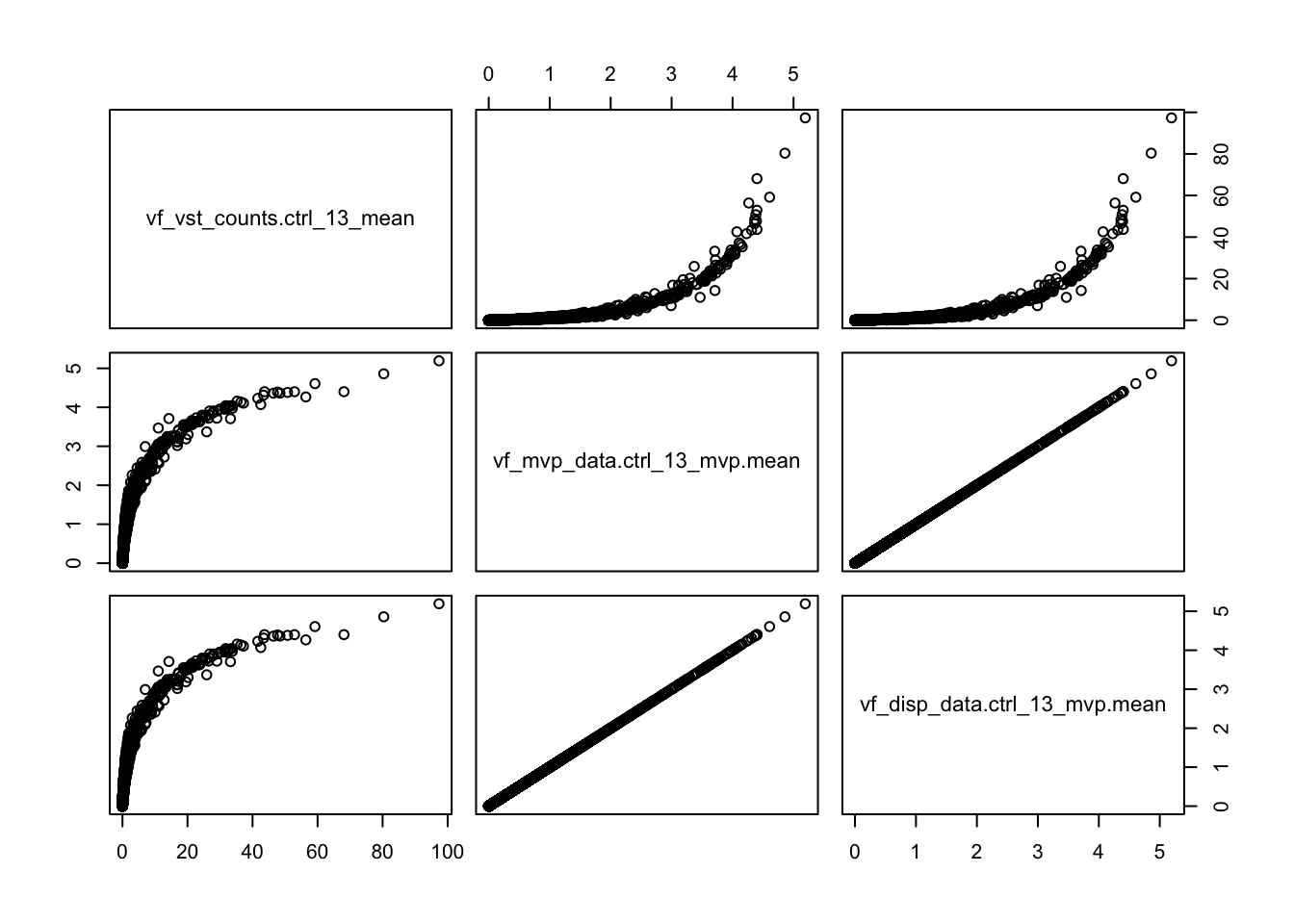
plot_hvg = function(df, m,d,vg, log=FALSE){
  top20 = head(vg,20)
  p = ggplot(df, aes(x=.data[[m]], y=.data[[d]], color=hvinfo)) + geom_point() + theme_classic()
  if (log) { p = p + scale_x_log10()}
  LabelPoints(plot = p, points = top20, repel = TRUE)
}

p1S =   plot_hvg(vinfo.seu, "vf_vst_counts.ctrl_13_mean", "vf_vst_counts.ctrl_13_variance.standardized",hvg_seu$vst, log=TRUE)
p2S =   plot_hvg(vinfo.seu, "vf_disp_data.ctrl_13_mvp.mean", "vf_disp_data.ctrl_13_mvp.dispersion.scaled",hvg_seu$disp)
p3S =   plot_hvg(vinfo.seu, "vf_mvp_data.ctrl_13_mvp.mean", "vf_mvp_data.ctrl_13_mvp.dispersion.scaled",hvg_seu$mvp)
wrap_plots(p1S,p2S,p3S,   ncol=2)
4.2 Bioc
Run the bioconductor detection method with modelGeneVar and getTopHVGs. Plot both total variance and “bio” variance.
ctrl.sce = as.SingleCellExperiment(ctrl)
var.out <- modelGeneVar(ctrl.sce)
hvgs_bioc <- getTopHVGs(var.out, n = 2000)

var.out.df = data.frame(var.out)
var.out.df$hvg = rownames(var.out) %in% hvgs_bioc
p = ggplot(var.out.df, aes(x=mean, y=total, colour = hvg)) + geom_point() + theme_classic()

top20 <- head(hvgs_bioc, 20)
pB = LabelPoints(plot = p, points = top20, repel = TRUE)
pB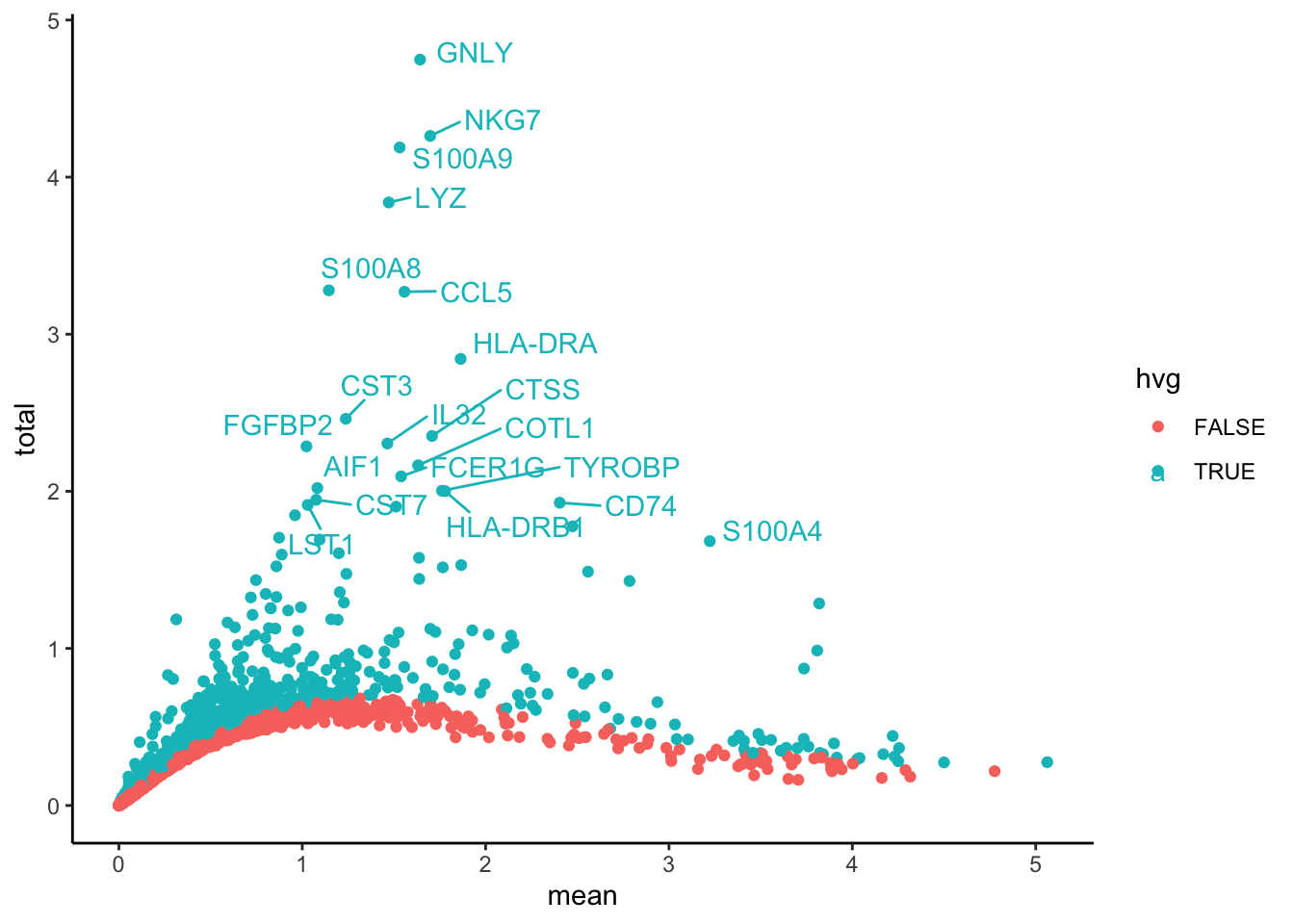
p2 = ggplot(var.out.df, aes(x=mean, y=bio, colour = hvg)) + geom_point() + theme_classic()

top20 <- head(hvgs_bioc, 20)
pB2 = LabelPoints(plot = p2, points = top20, repel = TRUE)
pB2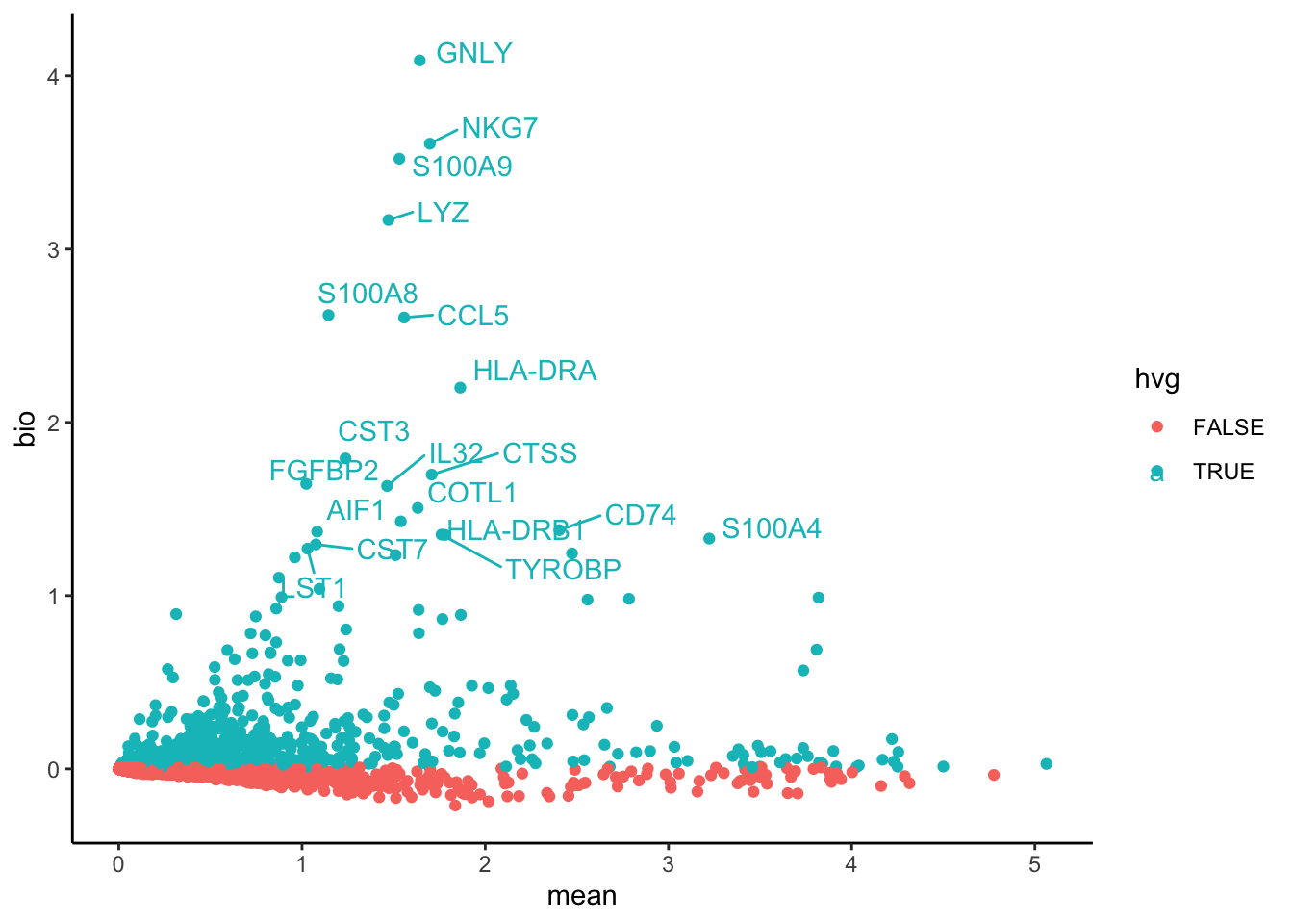
4.3 Scanpy
Run with both seurat (on lognorm data) and seurat_v3 (on counts, is same as vst)
For the dispersion-based methods (flavor=‘seurat’ Satija et al. [2015] and flavor=‘cell_ranger’ Zheng et al. [2017]), the normalized dispersion is obtained by scaling with the mean and standard deviation of the dispersions for genes falling into a given bin for mean expression of genes. This means that for each bin of mean expression, highly variable genes are selected.
For flavor=‘seurat_v3’/‘seurat_v3_paper’ [Stuart et al., 2019], a normalized variance for each gene is computed. First, the data are standardized (i.e., z-score normalization per feature) with a regularized standard deviation. Next, the normalized variance is computed as the variance of each gene after the transformation. Genes are ranked by the normalized variance. Only if batch_key is not None, the two flavors differ: For flavor=‘seurat_v3’, genes are first sorted by the median (across batches) rank, with ties broken by the number of batches a gene is a HVG. For flavor=‘seurat_v3_paper’, genes are first sorted by the number of batches a gene is a HVG, with ties broken by the median (across batches) rank.
penv = "/Users/asabjor/miniconda3/envs/scanpy_2024_nopip"
hvg.scanpy = basiliskRun(env=penv, fun=function(counts) {
    scanpy <- reticulate::import("scanpy")
    ad = reticulate::import("anndata")
    adata = ad$AnnData(counts)
    print(adata$X[1:10,1:10])
    var1 = scanpy$pp$highly_variable_genes(adata, flavor = "seurat_v3", inplace=FALSE)
    scanpy$pp$normalize_per_cell(adata, counts_per_cell_after=1e4)
    scanpy$pp$log1p(adata)
    print(adata$X[1:10,1:10])
    scanpy$pp$highly_variable_genes(adata)
    return(list(disp=adata$var, vst=var1))

}, counts = t(ctrl@assays$RNA@layers$counts.ctrl_13),  testload="scanpy")


#flavor
#Literal['seurat', 'cell_ranger', 'seurat_v3', 'seurat_v3_paper'] (default: 'seurat')rownames(hvg.scanpy$disp) = rownames(ctrl)
rownames(hvg.scanpy$vst) = rownames(ctrl)
top20 <- head(rownames(hvg.scanpy$disp)[order(hvg.scanpy$disp$dispersions_norm, decreasing = T)], 20)
p = ggplot(hvg.scanpy$disp, aes(x=means, y=dispersions_norm, colour = highly_variable)) + geom_point() + theme_classic() + ggtitle("Scanpy disp")
pS = LabelPoints(plot = p, points = top20, repel = TRUE)
pS 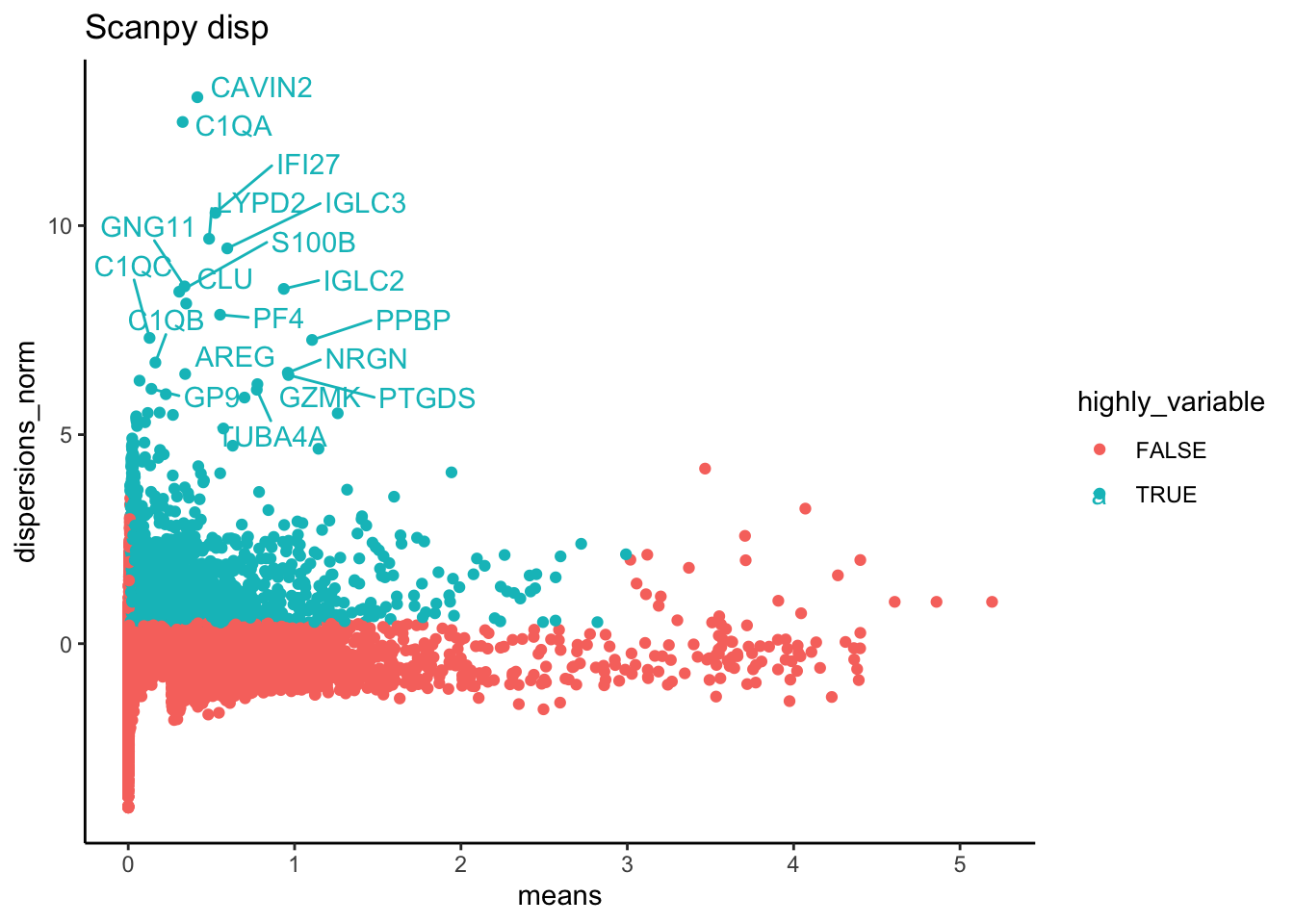
top20 <- head(rownames(hvg.scanpy$vst)[order(hvg.scanpy$vst$variances_norm, decreasing = T)], 20)
p2 = ggplot(hvg.scanpy$vst, aes(x=means, y=variances_norm, colour = highly_variable)) + geom_point() + theme_classic() + ggtitle("Scanpy vst") + scale_x_log10()

pS2 = LabelPoints(plot = p2, points = top20, repel = TRUE)
pS2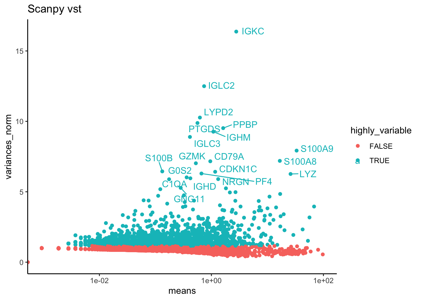
4.4 All together
colnames(hvg.scanpy$disp) = paste0(colnames(hvg.scanpy$disp), "_scpyD")
colnames(hvg.scanpy$vst) = paste0(colnames(hvg.scanpy$vst), "_scpyV")
colnames(var.out) = paste0(colnames(var.out), "_bioc")
ctrl.hvg = cbind(vinfo.seu, var.out, hvg.scanpy$disp, hvg.scanpy$vst)wrap_plots(p1S + ggtitle("Seurat vst"),p2S + ggtitle("Seurat disp"),p3S + ggtitle("Seurat mvp"),pB + ggtitle("Bioc total"),pS,pS2, ncol=3)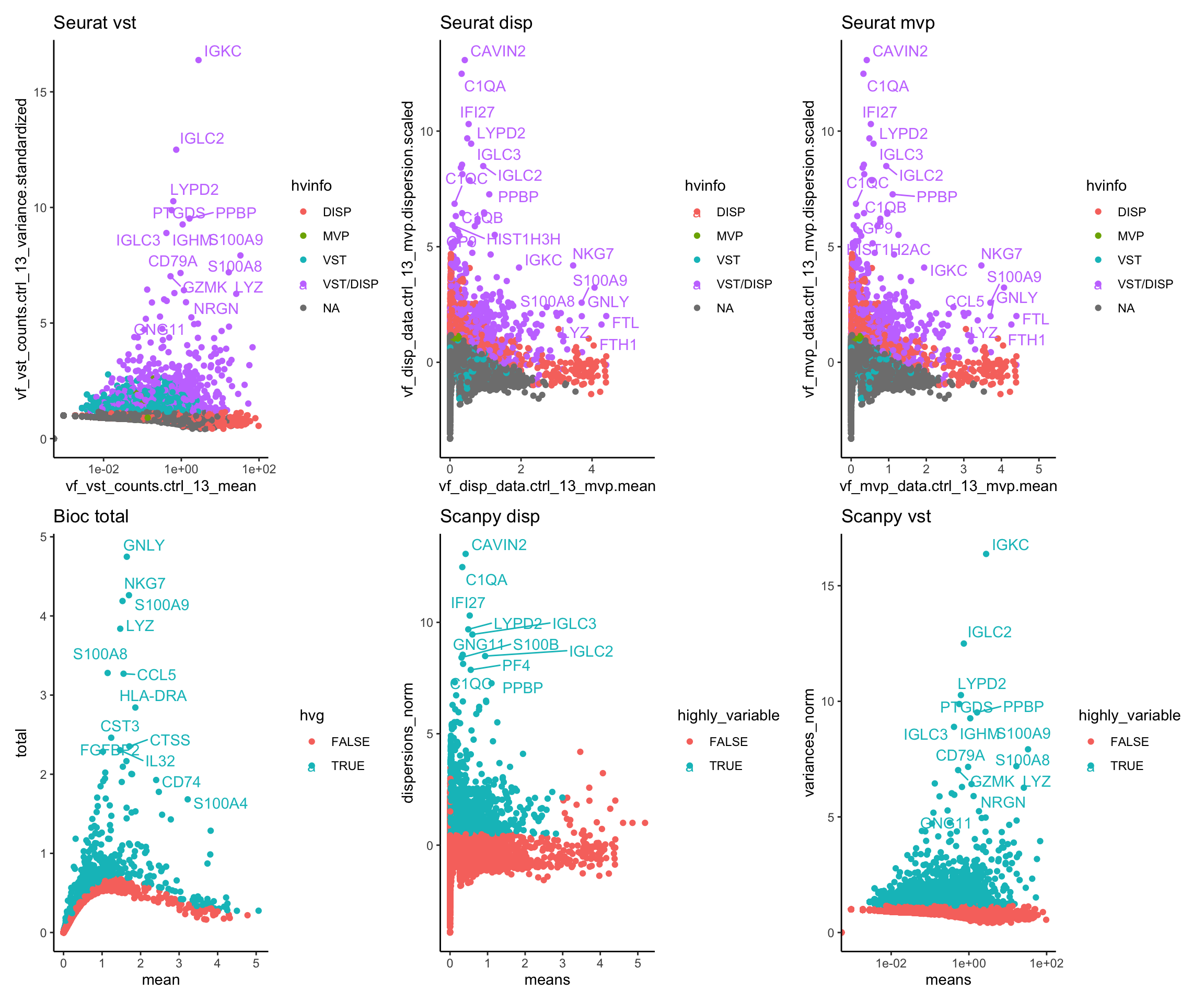
sel = c("vf_vst_counts.ctrl_13_variance.standardized","vf_disp_data.ctrl_13_mvp.dispersion.scaled","bio_bioc", "dispersions_norm_scpyD", "variances_norm_scpyV")

pairs(ctrl.hvg[,sel])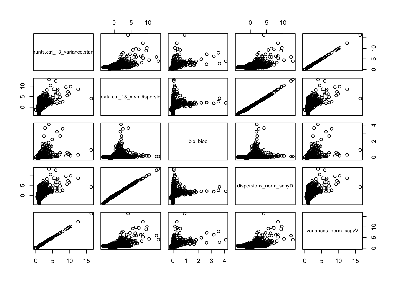
sel = c("vf_vst_counts.ctrl_13_mean_log","vf_disp_data.ctrl_13_mvp.mean", "mean_bioc", "means_scpyD", "means_scpyV_log")

ctrl.hvg$vf_vst_counts.ctrl_13_mean_log = log1p(ctrl.hvg$vf_vst_counts.ctrl_13_mean)
ctrl.hvg$means_scpyV_log = log1p(ctrl.hvg$means_scpyV)

pairs(ctrl.hvg[,sel])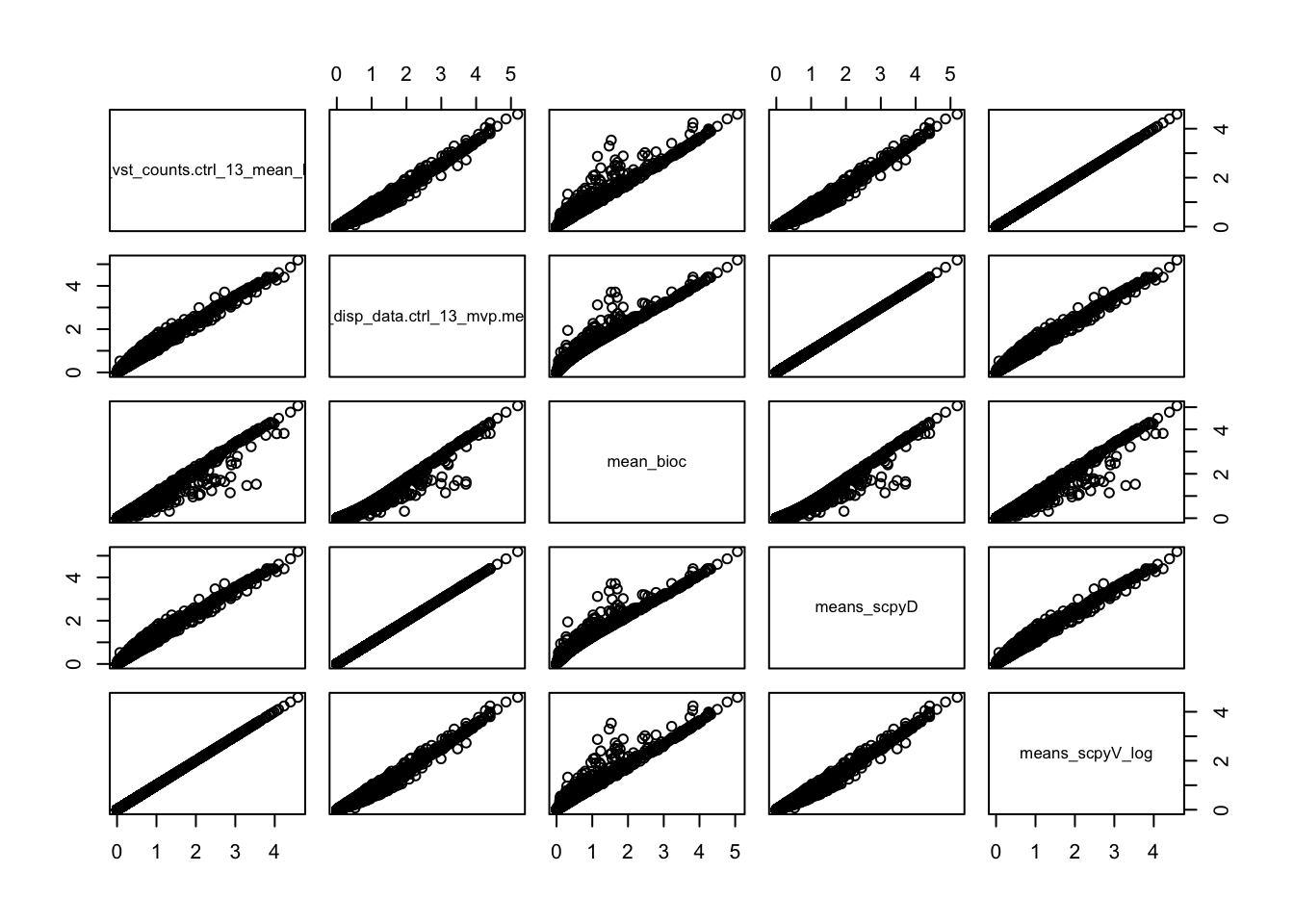
hvgs = hvg_seu
hvgs$scpyD = rownames(hvg.scanpy$disp)[hvg.scanpy$disp$highly_variable_scpyD]
hvgs$scpyV = rownames(hvg.scanpy$disp)[hvg.scanpy$vst$highly_variable_scpyV]
hvgs$bioc = hvgs_bioc

o = overlap_phyper2(hvgs,hvgs, remove.diag = T)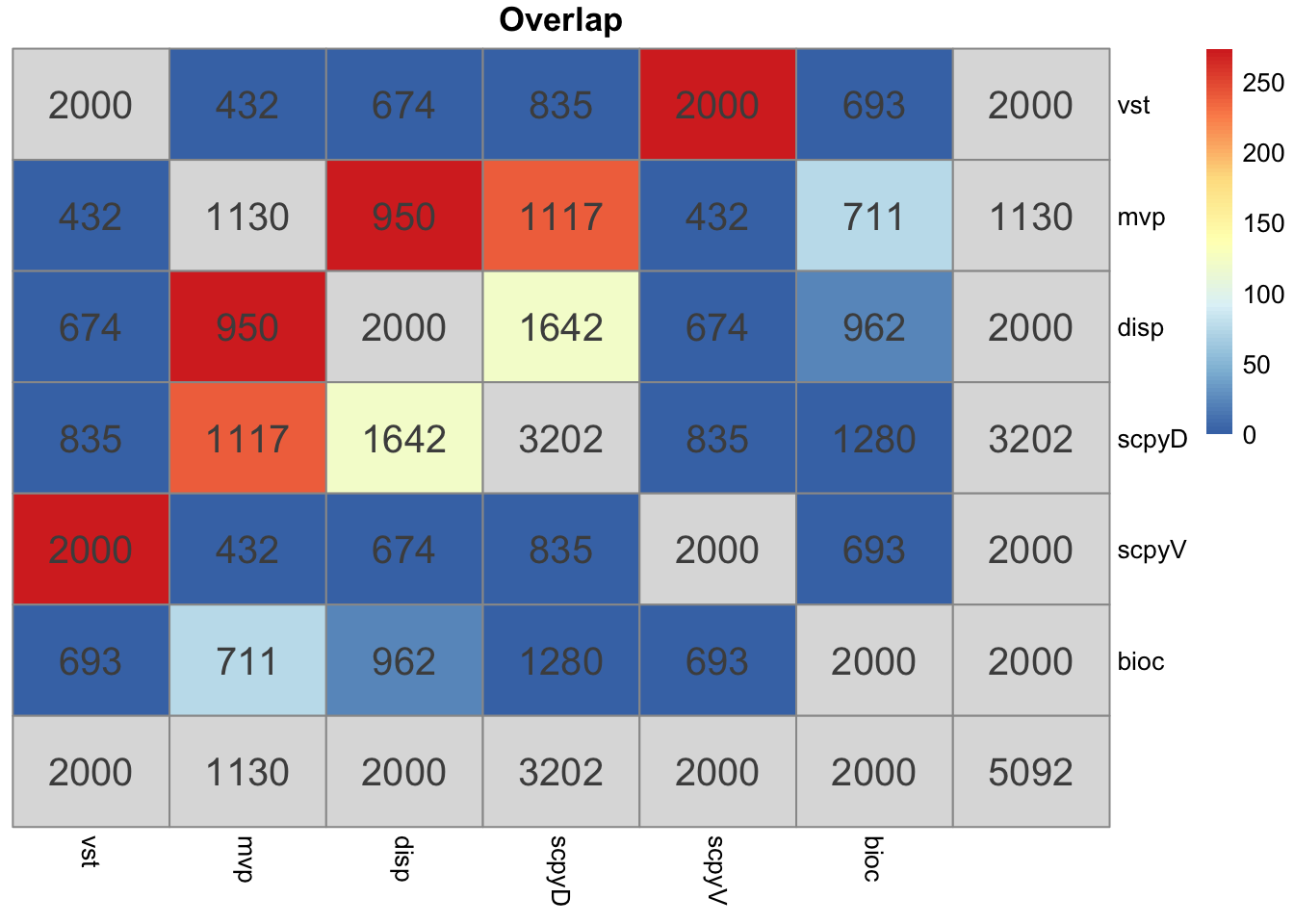
Mean Bioc stands out the most.
Vst in seurat and scanpy is identical and very different from the other methods. But it is also based on counts instead of lognorm data.
The variance estimate for the same sample is quite different. Even the top variable genes are not the same and are very different gene groups.
4.5 Top genes
Explore top genes with the different methods.
disp and mvp are identical, remove mvp.
ScanpyV and vst are identical, remove scpyV.
topG = lapply(hvgs, head, 10)

# same for mvp and disp, remove one of them.
topG$mvp = NULL
topG$scpyV = NULL

# sort the genes for scanpy.
topG$scpyD = rownames(ctrl.hvg)[order(ctrl.hvg$dispersions_norm_scpyD, decreasing = T)][1:10]


# rank the genes
allG = unique(unlist(topG))


ranks = Reduce(rbind, lapply(topG, function(x) {
  r = 1:10
  names(r) = x
  r2 = r[allG]
  return(r2)
}))

colnames(ranks) = allG
rownames(ranks) = names(topG)

pheatmap::pheatmap(ranks, display_numbers = ranks, main="Rank of top 10 gens", cluster_rows = F, cluster_cols = F)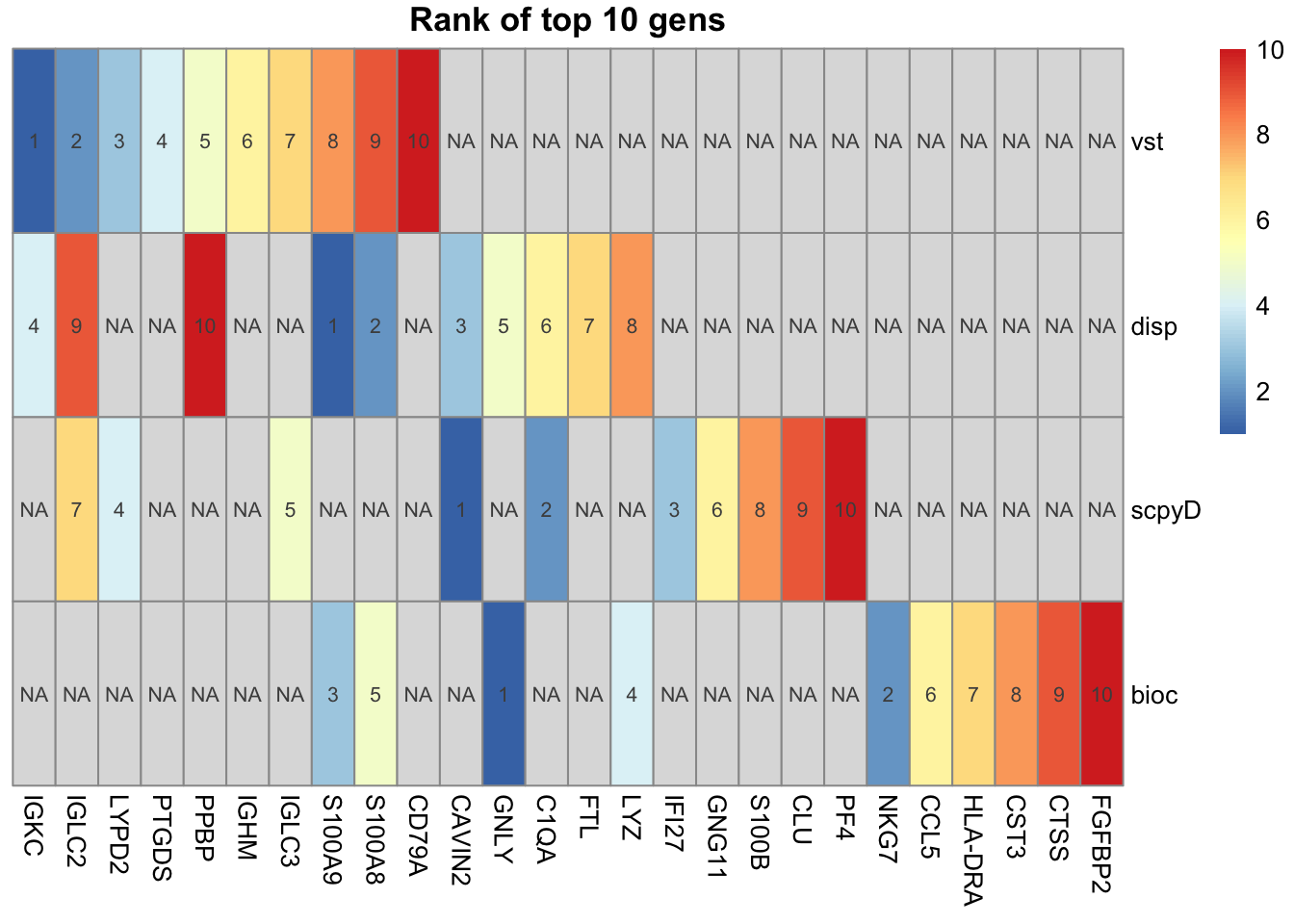
Plot onto umap for the unique ones.
topG$disp = NULL

t = table(unlist(topG))
selG = names(t)[t==1]
selG = sapply(selG, function(y) names(which(unlist(lapply(topG, function(x) any(x==y))))))
selG = sort(selG)

#small.leg <- theme(legend.text = element_text(size=3), legend.key.size = unit(0.5,"point"))

plots = list()
for (g in names(selG)){
  plots[[g]] = FeaturePlot(ctrl, reduction = "umap_harmony", features = g, order = T)  + ggtitle(paste(g,selG[g], collapse = " - ")) + NoAxes() #+ small.leg
}

wrap_plots(plots, ncol = 4)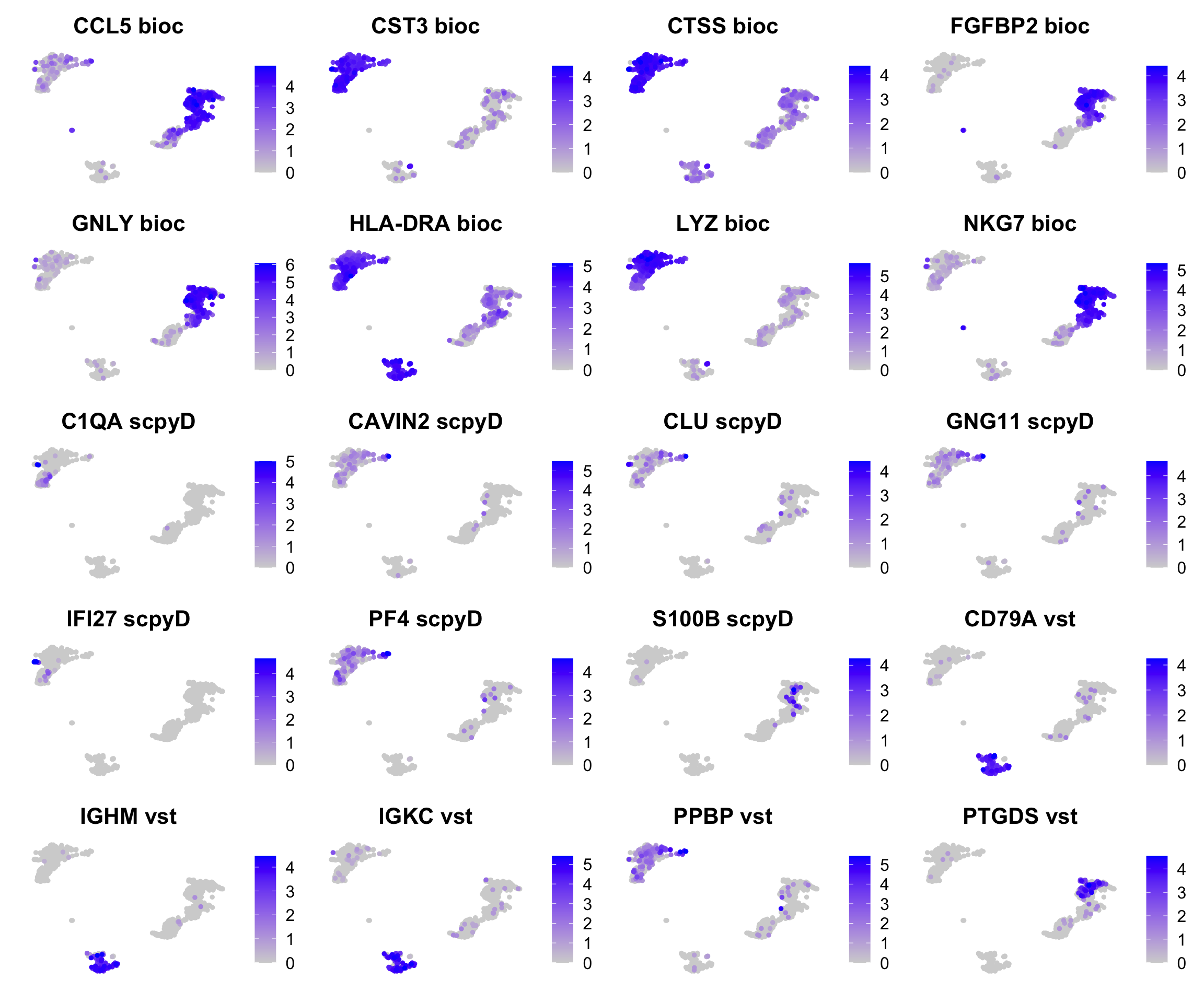
More clear celltype genes in the Bioc selection, but also higher expressed genes.. More B-cell genes for vst.
4.6 Expression levels
Expression levels of the variable genes. As total counts or mean expression across all cells.
ctrl.hvg$nC = rowSums(ctrl@assays$RNA@layers$counts.ctrl_13>0)
ctrl.hvg$meanE = rowMeans(ctrl@assays$RNA@layers$data.ctrl_13)
ctrl.hvg$vg_bioc = rownames(ctrl.hvg) %in% hvgs_bioc

wrap_plots(
ggplot(ctrl.hvg, aes(x=nC, fill=vg_vst)) + geom_histogram( alpha=0.5, position="identity") + scale_x_log10() + NoLegend() + ggtitle("VST"),
ggplot(ctrl.hvg, aes(x=nC, fill=vg_disp)) + geom_histogram( alpha=0.5, position="identity") + scale_x_log10() + NoLegend() + ggtitle("Disp"),
ggplot(ctrl.hvg, aes(x=nC, fill=highly_variable_scpyD)) + geom_histogram( alpha=0.5, position="identity") + scale_x_log10() + NoLegend() + ggtitle("Scanpy Disp"),
ggplot(ctrl.hvg, aes(x=nC, fill=highly_variable_scpyV)) + geom_histogram( alpha=0.5, position="identity") + scale_x_log10() + NoLegend() + ggtitle("Scanpy VST"),
ggplot(ctrl.hvg, aes(x=nC, fill=vg_bioc)) + geom_histogram( alpha=0.5, position="identity") + scale_x_log10() + NoLegend() + ggtitle("Bioc"),

ggplot(ctrl.hvg, aes(x=meanE, fill=vg_vst)) + geom_histogram( alpha=0.5, position="identity") + scale_x_log10() + NoLegend() + ggtitle("VST"),
ggplot(ctrl.hvg, aes(x=meanE, fill=vg_disp)) + geom_histogram( alpha=0.5, position="identity") + scale_x_log10() + NoLegend() + ggtitle("Disp"),
ggplot(ctrl.hvg, aes(x=meanE, fill=highly_variable_scpyD)) + geom_histogram( alpha=0.5, position="identity") + scale_x_log10() + NoLegend() + ggtitle("Scanpy Disp"),
ggplot(ctrl.hvg, aes(x=meanE, fill=highly_variable_scpyV)) + geom_histogram( alpha=0.5, position="identity") + scale_x_log10() + NoLegend() + ggtitle("Scanpy VST"),
ggplot(ctrl.hvg, aes(x=meanE, fill=vg_bioc)) + geom_histogram( alpha=0.5, position="identity") + scale_x_log10() + NoLegend()+ ggtitle("Bioc"),
ncol =5
)
BioC distibution shifted to more highly expressed genes.
Dispersion gives the very highly expressed genes, but also has a spread among all levels of expression.
5 Discussion
Seurat v3 paper suggests vst on counts, but then uses the variable genes in lognorm space, how is this the best option_
From SC best practices, suggests scry for HVG selection. https://www.sc-best-practices.org/preprocessing_visualization/feature_selection.html
5.1 scry
Run scry deviance function and select top 2k genes.
ctrl.sce<-scry::devianceFeatureSelection(ctrl.sce, assay="counts", sorted=TRUE)
plot(rowData(ctrl.sce)$binomial_deviance, type="l", xlab="ranked genes",
     ylab="binomial deviance", main="Feature Selection with Deviance")
abline(v=2000, lty=2, col="red")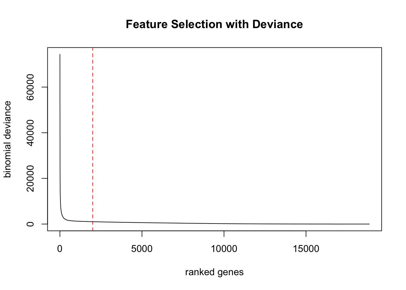
head(rowData(ctrl.sce),10)DataFrame with 10 rows and 1 column
binomial_deviance
<numeric>
S100A9 74343.0
FTL 53573.3
GNLY 52928.0
LYZ 48572.1
S100A8 42210.5
NKG7 36843.2
FTH1 35595.1
B2M 23773.7
CCL5 22340.5
HLA-DRA 21938.7Top genes are similar to the other methods.
ctrl.hvg$deviance = rowData(ctrl.sce)$binomial_deviance[match(rownames(ctrl.hvg), rownames(rowData(ctrl.sce)))]
ctrl.hvg$devG = rownames(ctrl.hvg) %in% head(rownames(rowData(ctrl.sce)),2000)

wrap_plots(
ggplot(ctrl.hvg, aes(x=nC, y=deviance, color=devG)) + geom_point() + theme_classic() + ggtitle("nCell vs deviance") + NoLegend(),
ggplot(ctrl.hvg, aes(x=meanE, y=deviance, color=devG)) + geom_point() + theme_classic() + ggtitle("mean expression vs deviance")+ NoLegend(),
ggplot(ctrl.hvg, aes(x=dispersions_norm_scpyD, y=deviance, color=devG)) + geom_point() + theme_classic() + ggtitle("Dispersion vs deviance")+ NoLegend(),
ggplot(ctrl.hvg, aes(x=variances_norm_scpyV, y=deviance, color=devG)) + geom_point() + theme_classic() + ggtitle("VST vs deviance")+ NoLegend(),
ggplot(ctrl.hvg, aes(x=bio_bioc, y=deviance, color=devG)) + geom_point() + theme_classic() + ggtitle("bioc bio vs deviance")+ NoLegend(),


ncol = 3
)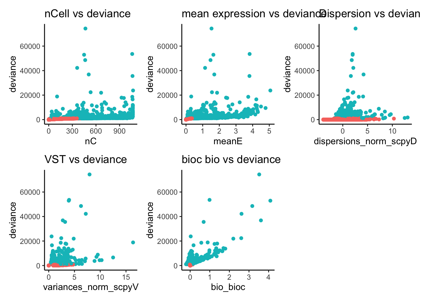
Selects all genes with high expression
hvgs$deviance = head(rownames(rowData(ctrl.sce)),2000)
o = overlap_phyper2(hvgs,hvgs, remove.diag = T)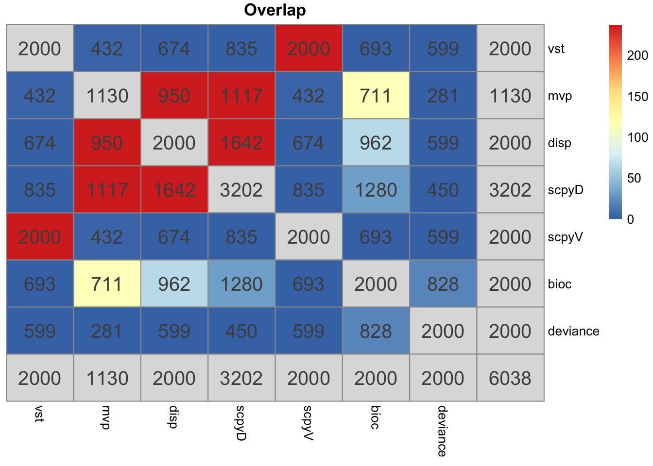
6 Session info
Click here
sessionInfo()R version 4.3.3 (2024-02-29)
Platform: x86_64-apple-darwin13.4.0 (64-bit)
Running under: macOS Big Sur ... 10.16
Matrix products: default
BLAS/LAPACK: /Users/asabjor/miniconda3/envs/seurat5_u/lib/libopenblasp-r0.3.28.dylib; LAPACK version 3.12.0
locale:
[1] sv_SE.UTF-8/sv_SE.UTF-8/sv_SE.UTF-8/C/sv_SE.UTF-8/sv_SE.UTF-8
time zone: Europe/Stockholm
tzcode source: system (macOS)
attached base packages:
[1] grid stats4 stats graphics grDevices utils datasets
[8] methods base
other attached packages:
[1] pheatmap_1.0.12 basilisk_1.14.1
[3] ComplexHeatmap_2.18.0 scran_1.30.0
[5] scuttle_1.12.0 SingleCellExperiment_1.24.0
[7] SummarizedExperiment_1.32.0 Biobase_2.62.0
[9] GenomicRanges_1.54.1 GenomeInfoDb_1.38.1
[11] IRanges_2.36.0 S4Vectors_0.40.2
[13] BiocGenerics_0.48.1 MatrixGenerics_1.14.0
[15] matrixStats_1.5.0 patchwork_1.3.0
[17] ggplot2_3.5.1 Matrix_1.6-5
[19] zellkonverter_1.12.1 Seurat_5.1.0
[21] SeuratObject_5.0.2 sp_2.1-4
loaded via a namespace (and not attached):
[1] RcppAnnoy_0.0.22 splines_4.3.3
[3] later_1.4.1 bitops_1.0-9
[5] filelock_1.0.3 tibble_3.2.1
[7] polyclip_1.10-7 basilisk.utils_1.14.1
[9] fastDummies_1.7.4 lifecycle_1.0.4
[11] doParallel_1.0.17 edgeR_4.0.16
[13] globals_0.16.3 lattice_0.22-6
[15] MASS_7.3-60.0.1 magrittr_2.0.3
[17] limma_3.58.1 plotly_4.10.4
[19] rmarkdown_2.29 remotes_2.5.0
[21] yaml_2.3.10 metapod_1.10.0
[23] httpuv_1.6.15 sctransform_0.4.1
[25] spam_2.11-0 sessioninfo_1.2.2
[27] pkgbuild_1.4.5 spatstat.sparse_3.1-0
[29] reticulate_1.40.0 cowplot_1.1.3
[31] pbapply_1.7-2 RColorBrewer_1.1-3
[33] pkgload_1.4.0 abind_1.4-5
[35] zlibbioc_1.48.0 Rtsne_0.17
[37] purrr_1.0.2 RCurl_1.98-1.16
[39] circlize_0.4.16 GenomeInfoDbData_1.2.11
[41] ggrepel_0.9.6 scry_1.14.0
[43] irlba_2.3.5.1 listenv_0.9.1
[45] spatstat.utils_3.1-2 goftest_1.2-3
[47] RSpectra_0.16-2 spatstat.random_3.3-2
[49] dqrng_0.3.2 fitdistrplus_1.2-2
[51] parallelly_1.41.0 DelayedMatrixStats_1.24.0
[53] leiden_0.4.3.1 codetools_0.2-20
[55] DelayedArray_0.28.0 shape_1.4.6.1
[57] tidyselect_1.2.1 farver_2.1.2
[59] ScaledMatrix_1.10.0 spatstat.explore_3.3-4
[61] jsonlite_1.8.9 GetoptLong_1.0.5
[63] BiocNeighbors_1.20.0 ellipsis_0.3.2
[65] progressr_0.15.1 iterators_1.0.14
[67] ggridges_0.5.6 survival_3.8-3
[69] foreach_1.5.2 tools_4.3.3
[71] ica_1.0-3 Rcpp_1.0.13-1
[73] glue_1.8.0 gridExtra_2.3
[75] SparseArray_1.2.2 xfun_0.50
[77] usethis_3.1.0 dplyr_1.1.4
[79] withr_3.0.2 fastmap_1.2.0
[81] bluster_1.12.0 digest_0.6.37
[83] rsvd_1.0.5 R6_2.5.1
[85] mime_0.12 colorspace_2.1-1
[87] Cairo_1.6-2 scattermore_1.2
[89] tensor_1.5 spatstat.data_3.1-4
[91] tidyr_1.3.1 generics_0.1.3
[93] data.table_1.15.4 httr_1.4.7
[95] htmlwidgets_1.6.4 S4Arrays_1.2.0
[97] uwot_0.1.16 pkgconfig_2.0.3
[99] gtable_0.3.6 lmtest_0.9-40
[101] XVector_0.42.0 htmltools_0.5.8.1
[103] profvis_0.4.0 dotCall64_1.2
[105] clue_0.3-66 scales_1.3.0
[107] png_0.1-8 spatstat.univar_3.1-1
[109] knitr_1.49 rjson_0.2.23
[111] reshape2_1.4.4 curl_6.0.1
[113] nlme_3.1-165 cachem_1.1.0
[115] GlobalOptions_0.1.2 zoo_1.8-12
[117] stringr_1.5.1 KernSmooth_2.23-26
[119] parallel_4.3.3 miniUI_0.1.1.1
[121] pillar_1.10.1 vctrs_0.6.5
[123] RANN_2.6.2 urlchecker_1.0.1
[125] promises_1.3.2 BiocSingular_1.18.0
[127] beachmat_2.18.0 xtable_1.8-4
[129] cluster_2.1.8 evaluate_1.0.1
[131] cli_3.6.3 locfit_1.5-9.10
[133] compiler_4.3.3 rlang_1.1.4
[135] crayon_1.5.3 future.apply_1.11.2
[137] labeling_0.4.3 fs_1.6.5
[139] plyr_1.8.9 stringi_1.8.4
[141] viridisLite_0.4.2 deldir_2.0-4
[143] BiocParallel_1.36.0 munsell_0.5.1
[145] lazyeval_0.2.2 devtools_2.4.5
[147] spatstat.geom_3.3-4 dir.expiry_1.10.0
[149] RcppHNSW_0.6.0 sparseMatrixStats_1.14.0
[151] future_1.34.0 statmod_1.5.0
[153] shiny_1.10.0 ROCR_1.0-11
[155] memoise_2.0.1 igraph_2.0.3