Comparison of DGE results

force_rerun = FALSE
if (force_rerun){
  reticulate::use_condaenv("/Users/asabjor/miniconda3/envs/scanpy_2024_nopip/")
  reticulate::py_config()
}

Load libraries

suppressPackageStartupMessages({
    library(Seurat)
    library(Matrix)
    library(ggplot2)
    library(patchwork)
    library(dplyr)
    library(scran)
    library(basilisk)
    library(basilisk.utils)
    library(zellkonverter)
    library(ComplexHeatmap)
})


#source("~/projects/sc-devop/single_cell_R_scripts/overlap_phyper_v2.R")
devtools::source_url("https://raw.githubusercontent.com/asabjorklund/single_cell_R_scripts/main/overlap_phyper_v2.R")

Load data

path_results <- "data/covid/results"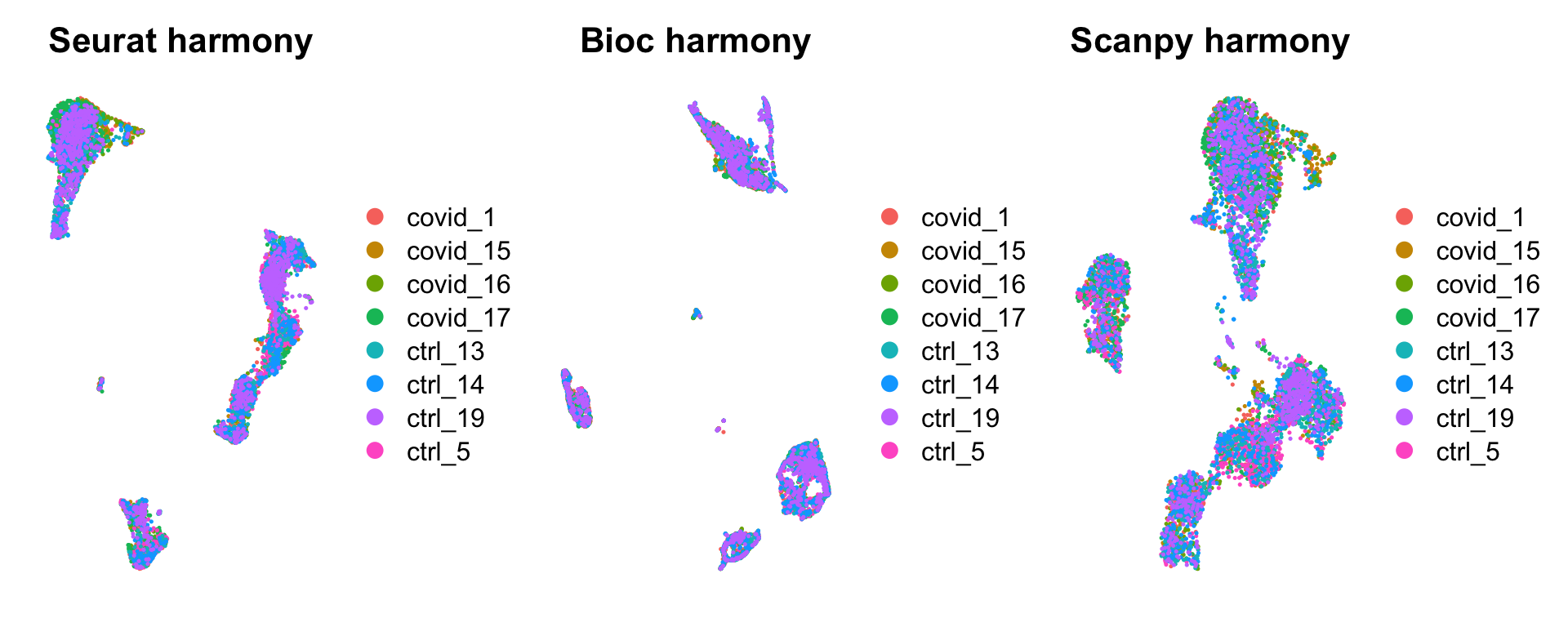
all = readRDS(file.path(path_results,"merged_all.rds"))

wrap_plots(
    DimPlot(all, group.by = "orig.ident", reduction = "umap_harmony") + NoAxes() + ggtitle("Seurat harmony"),
    DimPlot(all, group.by = "orig.ident", reduction = "umap_bioc_harmony") + NoAxes() + ggtitle("Bioc harmony"),
    DimPlot(all, group.by = "orig.ident", reduction = "umap_scpy_harmony") + NoAxes() + ggtitle("Scanpy harmony"),
    ncol = 3
)

Select one clustering and use that for DGE detection in all the different methods. Use clustering with Seurat and louvain_0.5.

sel.clust = "RNA_snn_res.0.5"

wrap_plots(
    DimPlot(all, group.by = sel.clust, reduction = "umap_harmony", label = T) + NoAxes() + ggtitle("Seurat harmony"),
    DimPlot(all, group.by = sel.clust, reduction = "umap_bioc_harmony", label = T) + NoAxes() + ggtitle("Bioc harmony"),
    DimPlot(all, group.by = sel.clust, reduction = "umap_scpy_harmony", label = T) + NoAxes() + ggtitle("Scanpy harmony"),
    ncol = 3
) + plot_layout(guides="collect")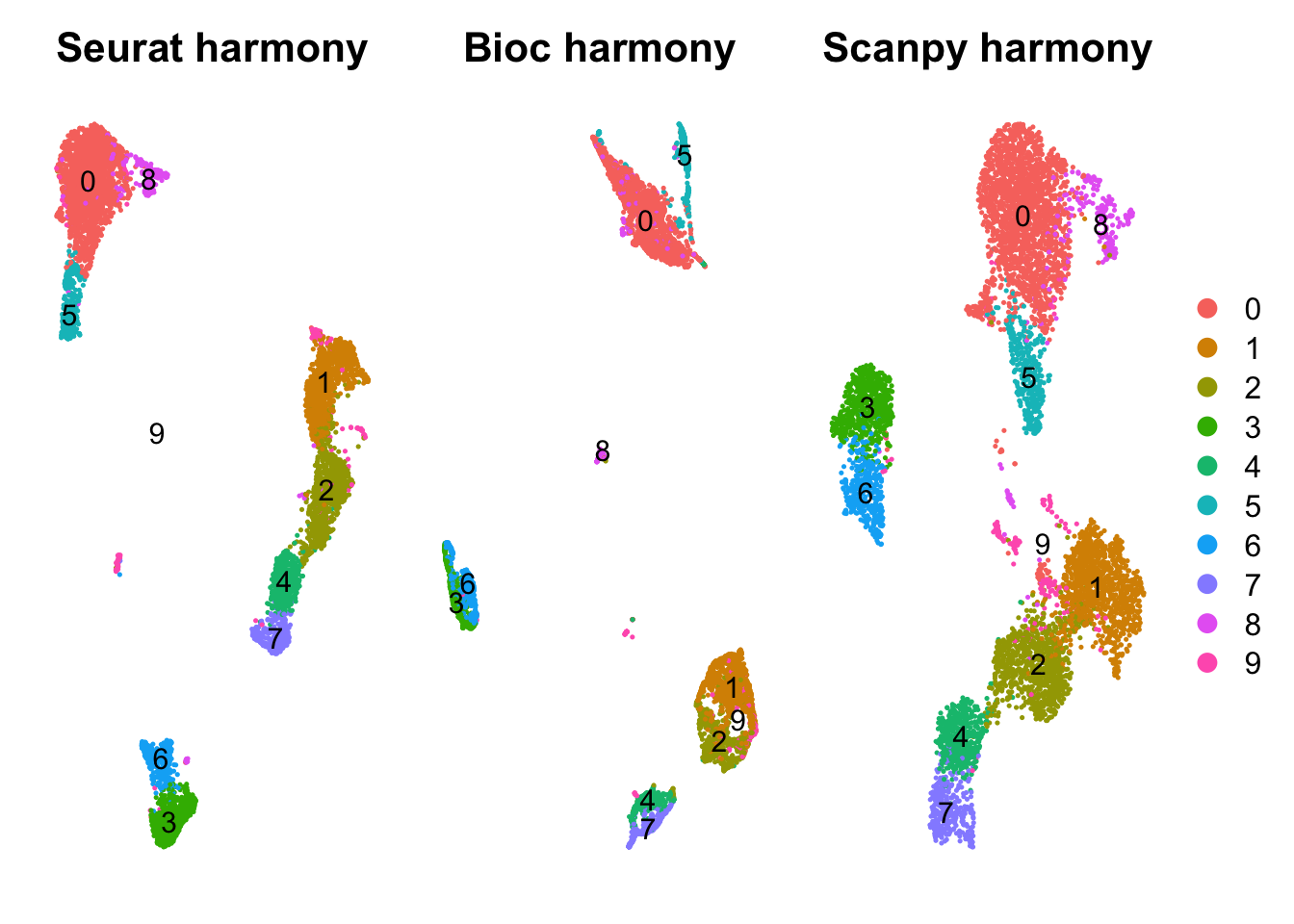

Rename clusters by celltypes to easier follow annotations.

• 0 - Mono/DC
• 1 - NK
• 2 - CD8T
• 3 - Bcell
• 4 - CD4T
• 5 - Mono
• 6 - Bcell
• 7 - CD4T
• 8 - unclear
• 9 - unclear

trans = c("M-0","NK-1","CD8-2","B-3","CD4-4","M-5","B-6","CD4-7","U-8","U-9")
names(trans) = as.character(0:9)

tmp = factor(trans[as.character(all[[sel.clust]][,1])], levels = sort(trans))
names(tmp) = colnames(all)

all$cluster = tmp
all = SetIdent(all, value = "cluster")


wrap_plots(
    DimPlot(all, group.by = "cluster", reduction = "umap_harmony", label = T) + NoAxes() + ggtitle("Seurat harmony"),
    DimPlot(all, group.by = "cluster", reduction = "umap_bioc_harmony", label = T) + NoAxes() + ggtitle("Bioc harmony"),
    DimPlot(all, group.by = "cluster", reduction = "umap_scpy_harmony", label = T) + NoAxes() + ggtitle("Scanpy harmony"),
    ncol = 3
) + plot_layout(guides="collect")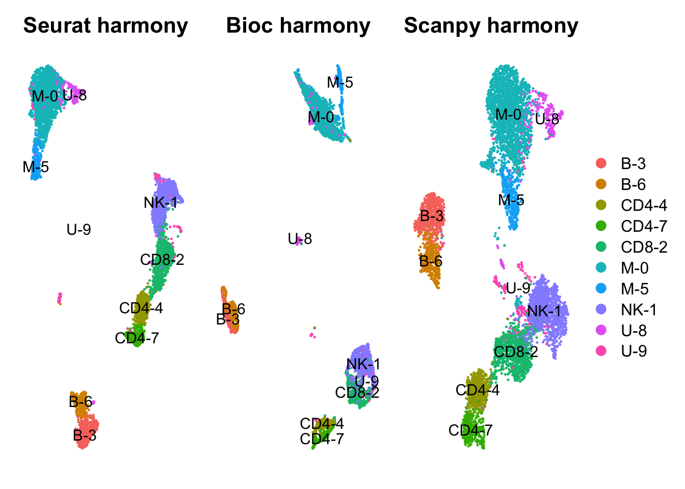

# Also merge the layers
all <- JoinLayers(object = all, layers = c("data","counts"))

0.1 Subsample

Subsample to 200 cells per cluster.

table(all@active.ident)

  B-3   B-6 CD4-4 CD4-7 CD8-2   M-0   M-5  NK-1   U-8   U-9 
  637   344   497   329   880  2078   335  1132   240   144 

all.sub = all[, WhichCells(all, downsample = 200)]
table(all.sub@active.ident)

  B-3   B-6 CD4-4 CD4-7 CD8-2   M-0   M-5  NK-1   U-8   U-9 
  200   200   200   200   200   200   200   200   200   144 

1 Seurat DGE

Run seurat FindAllMarkers with Wilcoxon, both the new implementation (wilcox) and similar to seurat v4 (wilcox_limma), MAST and T-test.

outfile = file.path(path_results, "seurat_dge.rds")
if (file.exists(outfile) & !force_rerun ){ 
  markersS = readRDS(outfile)
}else {

  markersS = list()
  markersS$wilc = FindAllMarkers(all.sub, test.use = "wilcox", only.pos = T)
  markersS$wilcL = FindAllMarkers(all.sub, test.use = "wilcox_limma", only.pos = T)
  markersS$Ttest = FindAllMarkers(all.sub, test.use = "t", only.pos = T)
  markersS$mast = FindAllMarkers(all.sub, test.use = "MAST", only.pos = T)
  saveRDS(markersS, file = outfile)
}

2 Bioc findMarkers

For Bioc no need to do the subsampling, if not for speed. It runs all pairwise comparisons and then combines the p-values across all tests.

Can run DGE with “all”, “some” and “any”.

• “any” - require significance in one pw test.
• “all” - dge in all pw tests. A
• “some” - combined p-value is calculated by taking the middlemost value of the Holm-corrected p-values for each gene. (By default, this the median for odd numbers of contrasts and one-after-the-median for even numbers, but the exact proportion can be changed by setting min.prop - see ?combineParallelPValues.) Here, the null hypothesis is that the gene is not DE in at least half of the contrasts.

If pval.type=“all”, the null hypothesis is that the gene is not DE in all contrasts. A combined p-value for each gene is computed using Berger’s intersection union test (IUT). Ranking based on the IUT p-value will focus on genes that are DE in that cluster compared to all other clusters. This strategy is particularly effective when dealing with distinct clusters that have a unique expression profile. In such cases, it yields a highly focused marker set that concisely captures the differences between clusters.

Still use the subsampled object for comparable numbers of cells.

Run with Wilcoxon, T-test and Binomial test.

sce = as.SingleCellExperiment(all.sub)

outfile = file.path(path_results, "bioc_dge.rds")
if (file.exists(outfile) & !force_rerun ){ 
  markersB = readRDS(outfile)
}else {

  markersB = list()
  markersB$wilc<- scran::findMarkers( sce, groups = sce$cluster,
    test.type = "wilcox", pval.type = "all",     direction = "up")

  markersB$Ttest<- scran::findMarkers( sce, groups = sce$cluster,
    test.type = "t", pval.type = "all",     direction = "up")

  markersB$binom<- scran::findMarkers( sce, groups = sce$cluster,
    test.type = "binom", pval.type = "all",     direction = "up")
  
  saveRDS(markersB, file = outfile)
}

outfile = file.path(path_results, "bioc_dge_some.rds")
if (file.exists(outfile) & !force_rerun ){ 
  markersBsome = readRDS(outfile)
}else {

  markersBsome = list()
  markersBsome$wilc<- scran::findMarkers( sce, groups = sce$cluster,
    test.type = "wilcox", pval.type = "some",     direction = "up")

  markersBsome$Ttest<- scran::findMarkers( sce, groups = sce$cluster,
    test.type = "t", pval.type = "some",     direction = "up")

  markersBsome$binom<- scran::findMarkers( sce, groups = sce$cluster,
    test.type = "binom", pval.type = "some",     direction = "up")
  
  saveRDS(markersBsome, file = outfile)
}

3 Bioc ScoreMarkers

From help section:

Compared to findMarkers, this function represents a simpler and more intuitive summary of the differences between the groups. We do this by realizing that the p-values for these types of comparisons are largely meaningless; individual cells are not meaningful units of experimental replication, while the groups themselves are defined from the data. Thus, by discarding the p-values, we can simplify our marker selection by focusing only on the effect sizes between groups.

Here, the strategy is to perform pairwise comparisons between each pair of groups to obtain various effect sizes. For each group X, we summarize the effect sizes across all pairwise comparisons involving that group, e.g., mean, min, max and so on. This yields a DataFrame for each group where each column contains a different summarized effect and each row corresponds to a gene in x. Reordering the rows by the summary of choice can yield a ranking of potential marker genes for downstream analyses.

outfile = file.path(path_results, "bioc_dge_score.rds")
if (file.exists(outfile) & !force_rerun ){ 
  markersBS = readRDS(outfile)
}else {
  markersBS <- scoreMarkers(sce, sce$cluster)
  saveRDS(markersBS, file = outfile)
}

Extract top ranked per cluster for mean.AUC, mean.logFC.cohen, mean.logFC.detected

The logFC.cohen columns contain the standardized log-fold change, i.e., Cohen’s d. For each pairwise comparison, this is defined as the difference in the mean log-expression for each group scaled by the average standard deviation across the two groups. (Technically, we should use the pooled variance; however, this introduces some unpleasant asymmetry depending on the variance of the larger group, so we take a simple average instead.) Cohen’s d is analogous to the t-statistic in a two-sample t-test and avoids spuriously large effect sizes from comparisons between highly variable groups. We can also interpret Cohen’s d as the number of standard deviations between the two group means.

The AUC columns contain the area under the curve. This is the probability that a randomly chosen observation in one group is greater than a randomly chosen observation in the other group. The AUC is closely related to the U-statistic used in the Wilcoxon rank sum test. Values greater than 0.5 indicate that a gene is upregulated in the first group.

The key difference between the AUC and Cohen’s d is that the former is less sensitive to the variance within each group

Finally, the logFC.detected columns contain the log-fold change in the proportion of cells with detected (i.e., non-zero) expression between groups.

Sstats = c("mean.AUC", "mean.logFC.cohen", "mean.logFC.detected")
names(Sstats) = c("bioc_AUC", "bioc_Cohen", "bioc_det")

clusters = levels(all$cluster)

rankedBS = list()
for (n in names(Sstats)){
  rankedBS[[n]] = list()
  for (cl in clusters){
    rankedBS[[n]][[cl]] = rownames(markersBS[[cl]])[order(markersBS[[cl]][,Sstats[n]], decreasing = TRUE)]
  }
}

4 Scanpy DGE

Running tests t-test, t-test_overestim_var, wilcoxon, logreg.

First, save SCE as an h5ad matrix. with zellkonverter. Then run python code with basilisk.

## Python code example
import scanpy 

fpath = "/Users/asabjor/courses/course_git/temp/workshop-scRNAseq/labs/comparison/data/covid/results/merged_all.h5ad"
adata = scanpy.read_h5ad(fpath)

print(adata.shape)
print(adata.X[1:10,1:10])

scanpy.pp.normalize_per_cell(adata, counts_per_cell_after=1e4)
scanpy.pp.log1p(adata)
print(adata.shape)
print(adata.X[1:10,1:10])
    
scanpy.tl.rank_genes_groups(adata, 'cluster', method='t-test', key_added = "Ttest")
print(adata.uns.Ttest.names[1:10])
scanpy$tl$rank_genes_groups(adata, 'cluster', method='t-test_overestim_var', key_added = "Ttest_o")
scanpy$tl$rank_genes_groups(adata, 'cluster', method='wilcoxon', key_added = "wilc")
scanpy$pp$scale(adata) # scale before logreg.
scanpy$tl$rank_genes_groups(adata, 'cluster', method='logreg', key_added = "logreg")

outfile = file.path(path_results, "scanpy_dge.rds")
if (file.exists(outfile) & !force_rerun ){ 
  dge.scanpy = readRDS(outfile)
}else {
zellkonverter::writeH5AD(sce, file.path(path_results,"merged_all.h5ad"))
reticulate::py_config()

penv = "/Users/asabjor/miniconda3/envs/scanpy_2024_nopip"
dge.scanpy = basiliskRun(env=penv, fun=function(fpath) {
    scanpy <- reticulate::import("scanpy")
    adata = scanpy$read_h5ad(fpath)
    
    output = list()
    output$shape1 = adata$shape
    output$head1 = adata$X[1:10,1:10]
    print(adata$shape)
    print(adata$X[1:10,1:10])
    scanpy$pp$normalize_per_cell(adata, counts_per_cell_after=1e4)
    scanpy$pp$log1p(adata)
    print(adata$shape)
    print(adata$X[1:10,1:10])
    output$shape2 = adata$shape
    output$head2 = adata$X[1:10,1:10]
    
    scanpy$tl$rank_genes_groups(adata, 'cluster', method='t-test', key_added = "Ttest")
    print(adata$uns['Ttest']['names'])
    scanpy$tl$rank_genes_groups(adata, 'cluster', method='t-test_overestim_var', key_added = "Ttest_o")
    scanpy$tl$rank_genes_groups(adata, 'cluster', method='wilcoxon', key_added = "wilc")
    scanpy$pp$scale(adata) # scale before logreg.
    scanpy$tl$rank_genes_groups(adata, 'cluster', method='logreg', key_added = "logreg")
    output$Ttest = adata$uns['Ttest']
    return(adata$uns)
    
}, fpath = "/Users/asabjor/courses/course_git/temp/workshop-scRNAseq/labs/comparison/data/covid/results/merged_all.h5ad",  testload="scanpy")
reticulate::py_config()

saveRDS(dge.scanpy, file = outfile)
}

Parse all scanpy results into dataframes

scanpy.tests = names(dge.scanpy)[-1:-2]
clusters = sort(unique(all$cluster))

# convert from lists to dfs.
markers_scanpy = list()
for (tname in scanpy.tests){
  x = dge.scanpy[[tname]]
  markers_scanpy[[tname]] = list()
  for (i in 1:length(clusters)){ 
    df = data.frame(Reduce(cbind, lapply(x[-1:-2], function(y) { y[,i]})))
    colnames(df) = names(x[-1:-2])
    rownames(df) = x$names[,i]
    markers_scanpy[[tname]][[i]] = df
  }
}

5 Compare significant genes.

Create a list object with all the significant dge genes.

• FDR from BioC findMarkers is the BH-adjusted p-value.
• Adjusted p-value from scanpy is BH-adjusted p-value. Scanpy logreg does not have p-values.
• P-values in Seurat are also BH.
• OBS! BioC scoreMarkers does not provide p-values in the same way, cannot compare here.

Not sure how they define the BH background, all genes, or genes after prefiltering.

Set cutoff for significant at 0.01.

pval.cut = 0.01

sign.scanpy = lapply(markers_scanpy, function(x) { 
  tmp = lapply(x, function(y) y[y$pvals_adj <= pval.cut,])
  names(tmp) = as.character(clusters) 
  return(tmp)
  })

sign.dge = unlist(sign.scanpy, recursive = F)
names(sign.dge) = sub("Ttest_o", "TtestO", names(sign.dge))
names(sign.dge) = paste0("scpy_", names(sign.dge))

sign.bioc = lapply(markersB, function(x) { 
  lapply(x, function(y) y[y$FDR <= pval.cut,])
  })
names(sign.bioc) = paste0("bioc_", names(sign.bioc))
sign.bioc = unlist(sign.bioc, recursive = F)

sign.biocS = lapply(markersBsome, function(x) { 
  lapply(x, function(y) y[y$FDR <= pval.cut,])
  })
names(sign.biocS) = paste0("bioc_SOME-", names(sign.biocS))
sign.biocS = unlist(sign.biocS, recursive = F)

sign.seu = lapply(markersS, function(x){
  x = x[x$p_val_adj <= pval.cut,]
  x = split(x, x$cluster)
  x = lapply(x, function(y) { 
    rownames(y) = y$gene
    return(y) })    
  x
})


names(sign.seu) = paste0("seu_", names(sign.seu))
sign.seu = unlist(sign.seu, recursive = F)

sign.dge = c(sign.dge, sign.seu, sign.bioc, sign.biocS)

saveRDS(sign.dge, file = file.path(path_results, "all_sign_dge.Rds"))

Number of dge genes

nG = unlist(lapply(sign.dge, nrow))
pipeline = Reduce(rbind,strsplit(names(nG),"_"))[,1]
par(mar = c(8,5,2,2))
barplot(nG, las = 2, col = factor(pipeline), main = "Number of significant genes", cex.names = 0.5)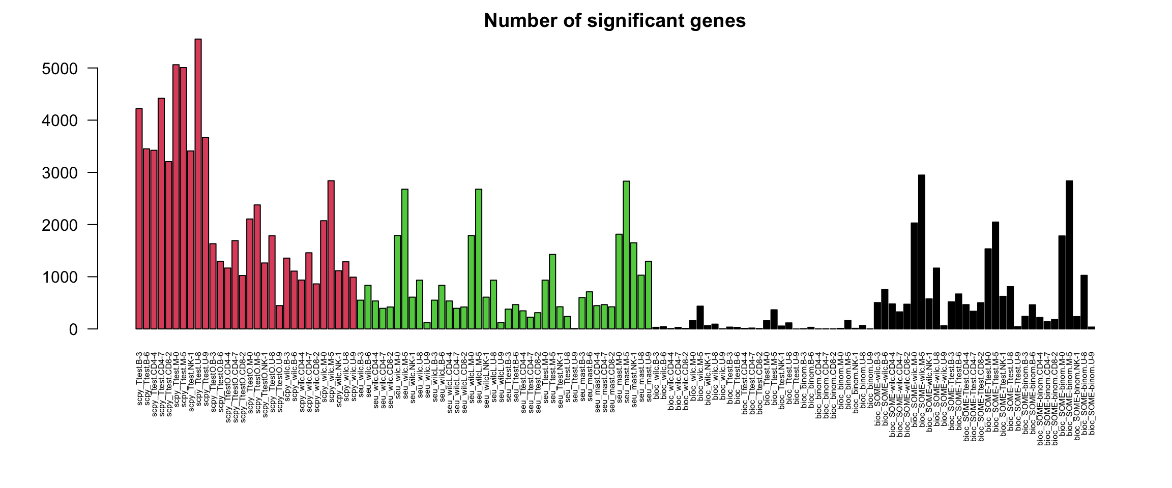

Turns out that the two different wilcoxon runs in Seurat have identical results, so remove one. sign.dge

Overlap of DGE genes is calculated with a phyper test using all expressed genes as the background. The heatmaps display the -log10(p-value) from the phyper test.

sign.dge = sign.dge[!grepl("wilcL",names(sign.dge))]

tmp = lapply(sign.dge, rownames)
o = overlap_phyper2(tmp, tmp, nsize = 5, bg = nrow(all), remove.diag = T, silent = T)

# Cluster and plot with annotation.

n = names(sign.dge)

s = Reduce(rbind, strsplit(n, "[\\._]"))
annot.tests = data.frame(s)
colnames(annot.tests) = c("Pipe","Test","Cluster")
rownames(annot.tests) = names(sign.dge)
annot.tests$TestName = paste(s[,1],s[,2], sep= "_")

pheatmap(-log10(o$P[1:100,1:100]+1e-230),annotation_col = annot.tests, fontsize = 6)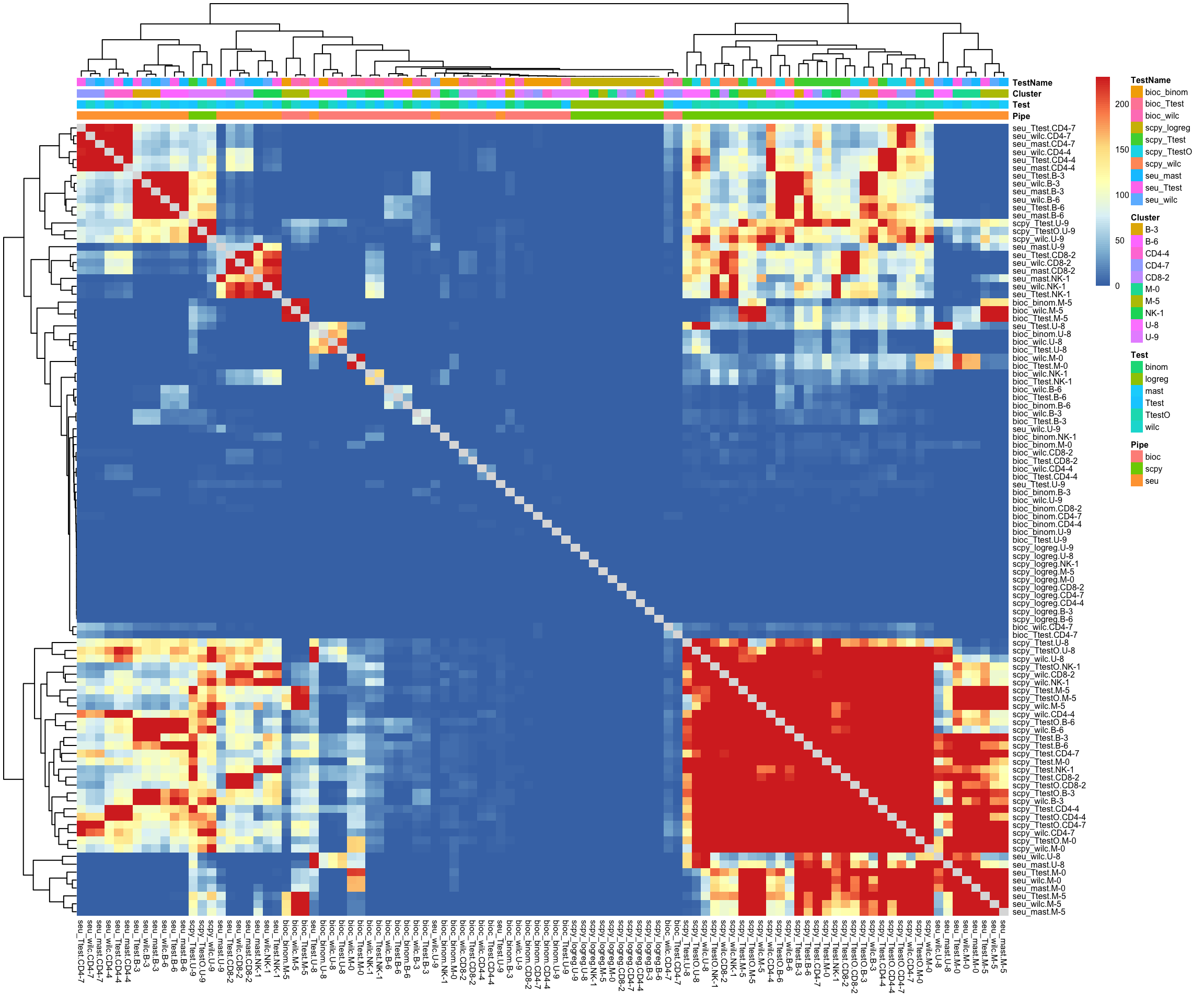

Mainly grouping by test. Very different number of genes, so unfair comparison for the scanpy tests.

6 Compare top genes

Create a list object with all the dge genes as ranked lists to compare top X genes.

ranked.scanpy = lapply(markers_scanpy, function(x) { 
  tmp = lapply(x, rownames)
  names(tmp) = clusters
  return(tmp)
  })

names(ranked.scanpy) = paste0("scpy_", names(ranked.scanpy))
names(ranked.scanpy) = sub("Ttest_o", "TtestO", names(ranked.scanpy))
ranked.scanpy = unlist(ranked.scanpy, recursive = F)


getRankSeu = function(x) {
  x = split(x, x$cluster)
  lapply(x, function(y) { 
    y$gene } )
}

rank.seu = lapply(markersS, getRankSeu)
names(rank.seu) = paste0("seu_", names(rank.seu))
rank.seu = unlist(rank.seu, recursive = F)

# remove wilcoxonL
rank.seu = rank.seu[!grepl("wilcL", names(rank.seu))]


rank.bioc = lapply(markersB, function(x) { 
  lapply(x, rownames)
})
names(rank.bioc) = paste0("bioc_", names(rank.bioc))
rank.bioc = unlist(rank.bioc, recursive = F)

rank.biocSOME = lapply(markersBsome, function(x) { 
  lapply(x, rownames)
})
names(rank.biocSOME) = paste0("bioc_SOME-", names(rank.biocSOME))
rank.biocSOME = unlist(rank.biocSOME, recursive = F)

rank.biocS = unlist(rankedBS, recursive = F)

all.rank = c(ranked.scanpy, rank.seu, rank.bioc, rank.biocSOME,rank.biocS )

saveRDS(all.rank, file = file.path(path_results, "all_ranked_dge.Rds"))

6.1 Top 50

n = names(all.rank)
s = Reduce(rbind, strsplit(n, "[\\._]"))
annot.tests = data.frame(s)
colnames(annot.tests) = c("Pipe","Test","Cluster")
rownames(annot.tests) = n
annot.tests$TestName = paste(s[,1],s[,2], sep= "_")


topG = lapply(all.rank, function(x) x[1:50])

o = overlap_phyper2(topG,topG, nsize = 5, bg = nrow(all), remove.diag = T, silent = T)
pvals = o$P[1:(ncol(o$P)-1), 1:(ncol(o$P)-1)]

pheatmap(-log10(pvals+1e-320),annotation_col = annot.tests, fontsize = 6)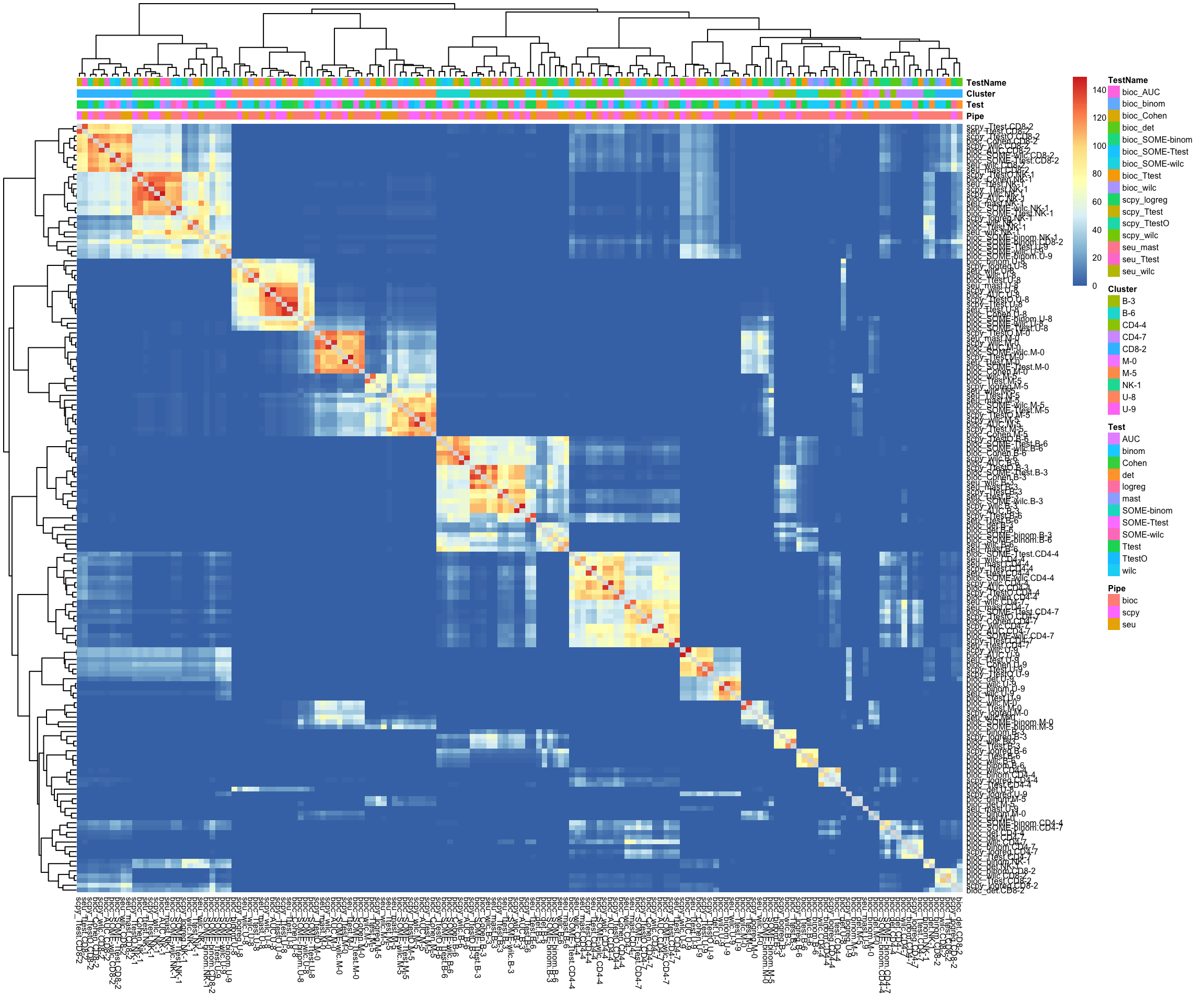

Mainly grouping by cluster now, the bioC methods stand out quite a bit.

Clearly more unique genes per cluster with the bioC methods.

Merge all top genes from all clusters.

OBS! Skip using background, all overlaps are significant, so we will get a false scale of the p-values, but is more visual.

tmp = split(topG, annot.tests$TestName)
tmp = lapply(tmp, unlist)
tmp = lapply(tmp, unique)

o = overlap_phyper2(tmp,tmp, remove.diag = T, silent = T)

# with grouping.
pheatmap(-log10(o$P + 1e-320)[1:length(tmp), 1:length(tmp)], display_numbers = o$M[1:length(tmp), 1:length(tmp)])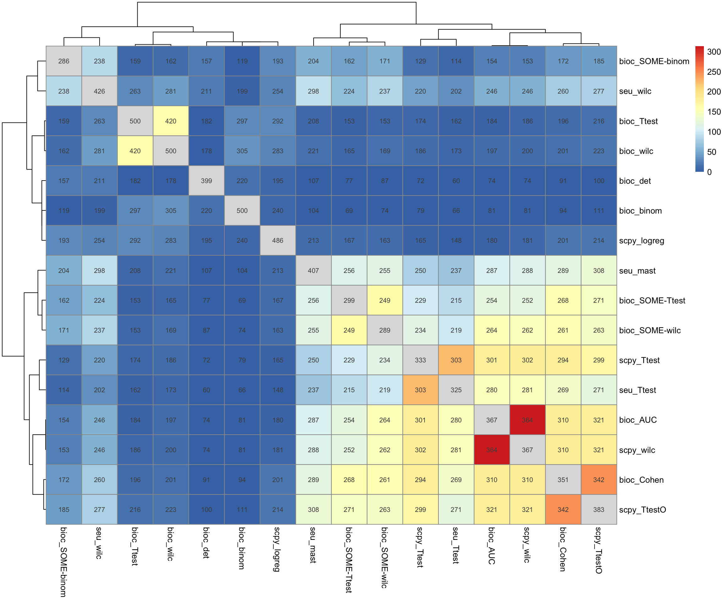

All bioc ScoreMarker test with unique genes stands out. But with “SOME” it overlaps more.

Surprisingly low overlap for scanpy and seurat wilcoxon test.

6.2 Top 200

Same but with top200 genes.

topG = lapply(all.rank, function(x) x[1:200])
tmp = split(topG, annot.tests$TestName)
tmp = lapply(tmp, unlist)
tmp = lapply(tmp, unique)

o = overlap_phyper2(tmp,tmp, remove.diag = T, silent = T)

# with grouping.
pheatmap(-log10(o$P + 1e-320)[1:length(tmp), 1:length(tmp)], display_numbers = o$M[1:length(tmp), 1:length(tmp)])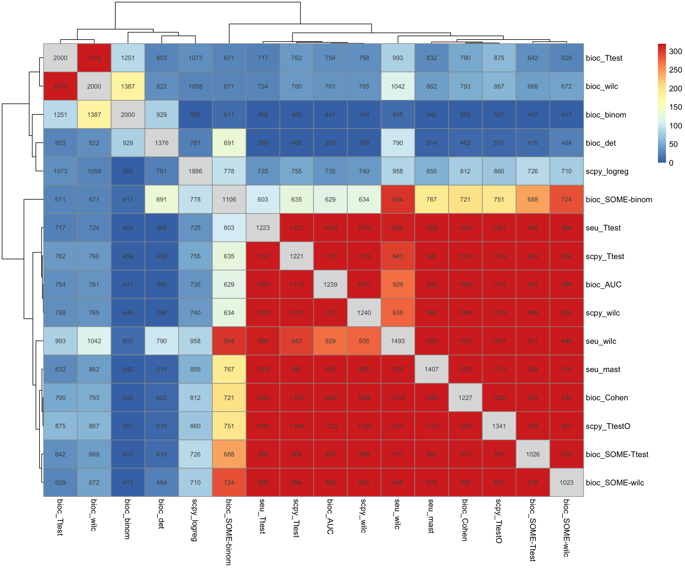

BioC stands out from the rest. Wilcoxon in Seurat and Scanpy are different.

6.3 Expression distribution

Expression distribution of the top 200 genes, both as number of cells expressed or as mean lognorm expression.

stats.df = data.frame(row.names = rownames(all.sub))
stats.df$nC = rowSums(all.sub@assays$RNA@layers$counts>0)
stats.df$meanE = rowMeans(all.sub@assays$RNA@layers$data)

# remove non-expressed genes
stats.df = stats.df[stats.df$nC>0 & stats.df$meanE > 0,]

top200 = tmp
for (n in names(tmp)){
  stats.df[[n]] = rownames(stats.df) %in% tmp[[n]]
}

Number of cells detected.

plots = list()
plots$all = ggplot(stats.df, aes(x=nC)) + geom_histogram( alpha=0.5, position="identity", binwidth = 0.05)  + scale_x_log10(limits = c(0.9,2000)) + NoLegend() + ggtitle("All genes") 
for (n in names(tmp)){
  plots[[n]] = ggplot(stats.df[stats.df[,n],], aes(x=nC)) + geom_histogram( alpha=0.5, position="identity", binwidth=0.05) + scale_x_log10(limits = c(0.9,2000)) + NoLegend() + ggtitle(n) 
}

wrap_plots(plots, ncol=4)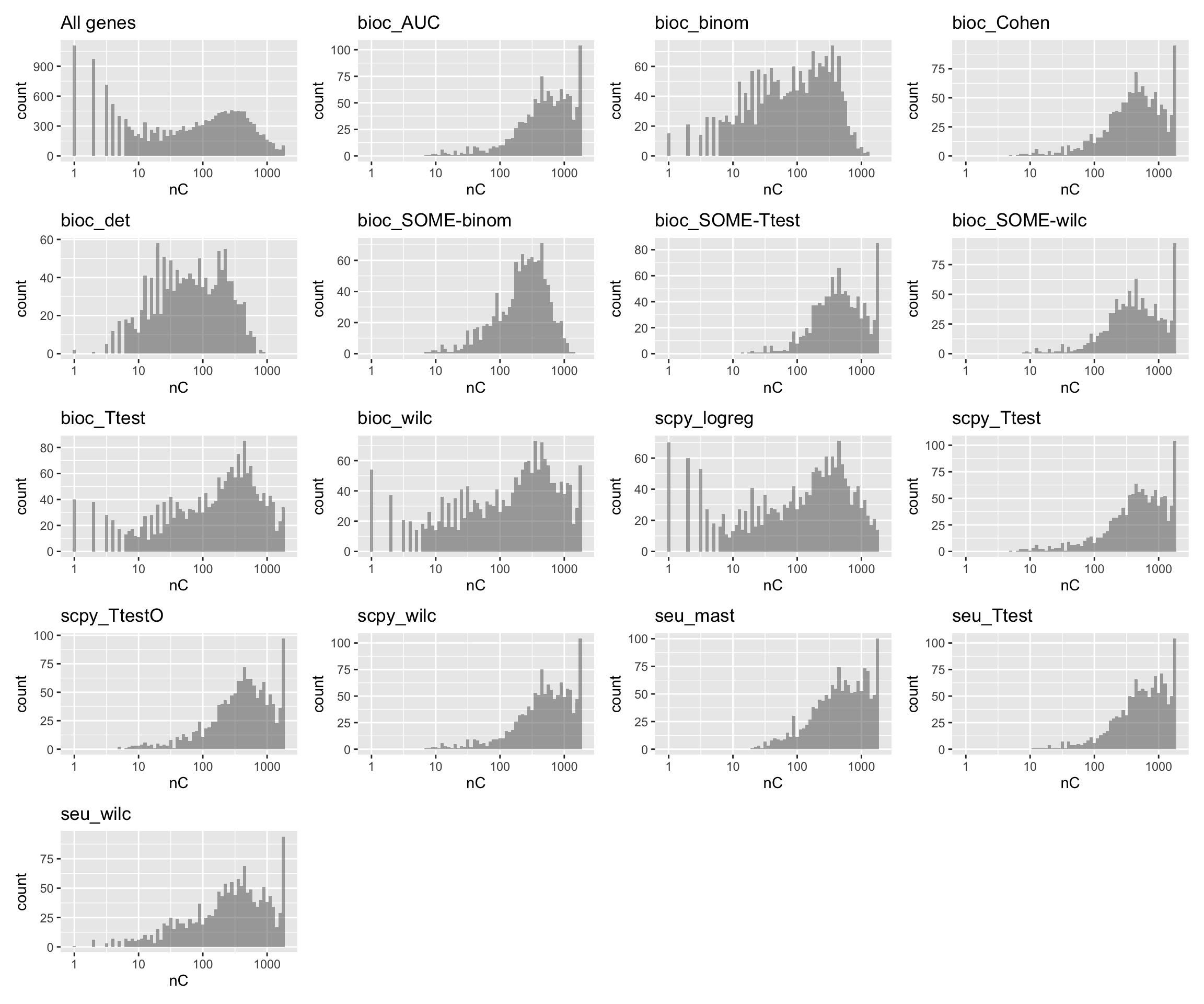

Mean expression

plots = list()
plots$all = ggplot(stats.df, aes(x=meanE)) + geom_histogram( alpha=0.5, position="identity", binwidth = 0.05)  + scale_x_log10(limits = c(0.0001,5)) + NoLegend() + ggtitle("All genes") +RotatedAxis()
for (n in names(tmp)){
  plots[[n]] = ggplot(stats.df[stats.df[,n],], aes(x=meanE)) + geom_histogram( alpha=0.5, position="identity", binwidth=0.05) + scale_x_log10(limits = c(0.0001,5)) + NoLegend() + ggtitle(n) + RotatedAxis()
}

wrap_plots(plots, ncol=4)

7 For one cluster

Select one cluster and compare the DGEs for that cluster across all methods. Use one of the CD4 clusters.

7.0.1 CD4-7

clust = "CD4-7"
sel = which(annot.tests$Cluster == clust)
ranked.sel = all.rank[sel]

Top 50 genes:

topG = lapply(ranked.sel, function(x) x[1:50])

o = overlap_phyper2(topG,topG, nsize = 5, bg = nrow(all), remove.diag = T)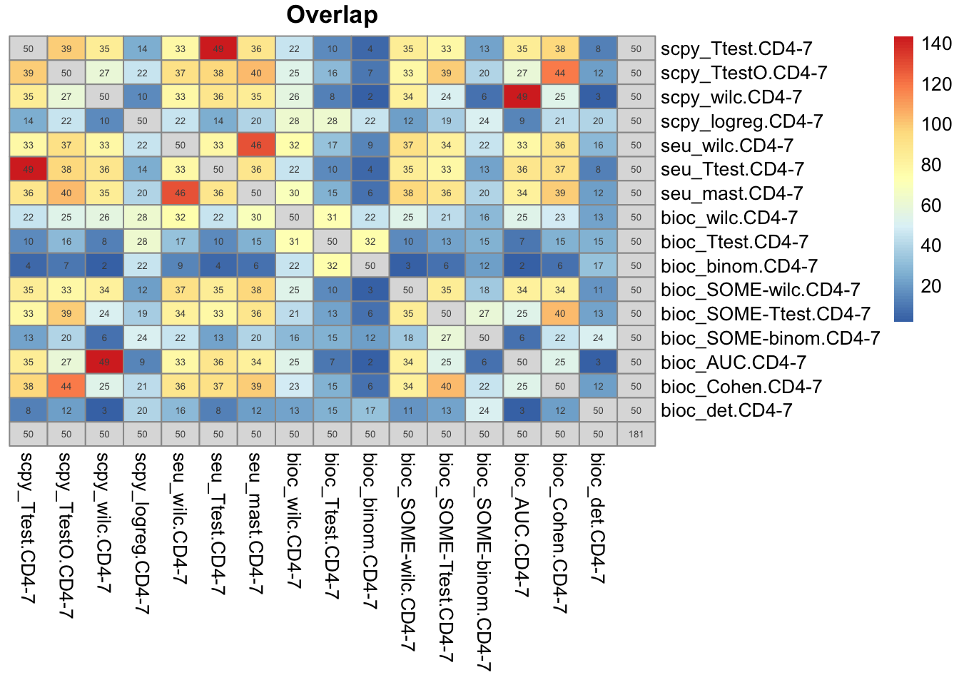

head(sort(table(unlist(topG)),decreasing = T),10)

   CCR7    LEF1 PIK3IP1    TCF7 TRABD2A  GIMAP7    IL7R   RPLP2    RPS6   SATB1 
     16      16      14      14      14      13      13      12      12      12 

Only 2 genes selected in all 16 tests.

Instead take top 10 genes and plot expression levels and sidebar with presence/absence in top10 list:

topG = lapply(ranked.sel, function(x) x[1:10])

gene_overlap_heatmap = function(topG){ 

  genes = sort(unique(unlist(topG)))

  tmp = all.sub[genes,]
  D = as.matrix(tmp@assays$RNA@layers$data)
  rownames(D) = genes 
  colnames(D) = colnames(all.sub)
  # reorder D
  D = D[,order(all.sub$cluster)]
  
  coldef = c("red","blue")
  names(coldef) = c("FALSE","TRUE")
  
  annotG = data.frame(row.names = genes)
  annot.col = list()
  for (n in names(topG)){
    annotG[[n]] = as.character(rownames(annotG) %in% topG[[n]])
    annot.col[[n]] = coldef
  }  
  
  annotC = data.frame(cluster=all.sub$cluster)
  rownames(annotC) = colnames(all.sub)
  
  coldef = c("blue","red")
  names(coldef) = c("TRUE","FALSE")
  cols2 <- RColorBrewer::brewer.pal(10, "Set3")
  names(cols2) = clusters
  coldef = c(coldef, cols2)

  pheatmap(D, annotation_row = annotG, cluster_cols = F, cluster_rows = T, labels_col = F, annotation_colors = annot.col, annotation_col = annotC)
}

gene_overlap_heatmap(topG)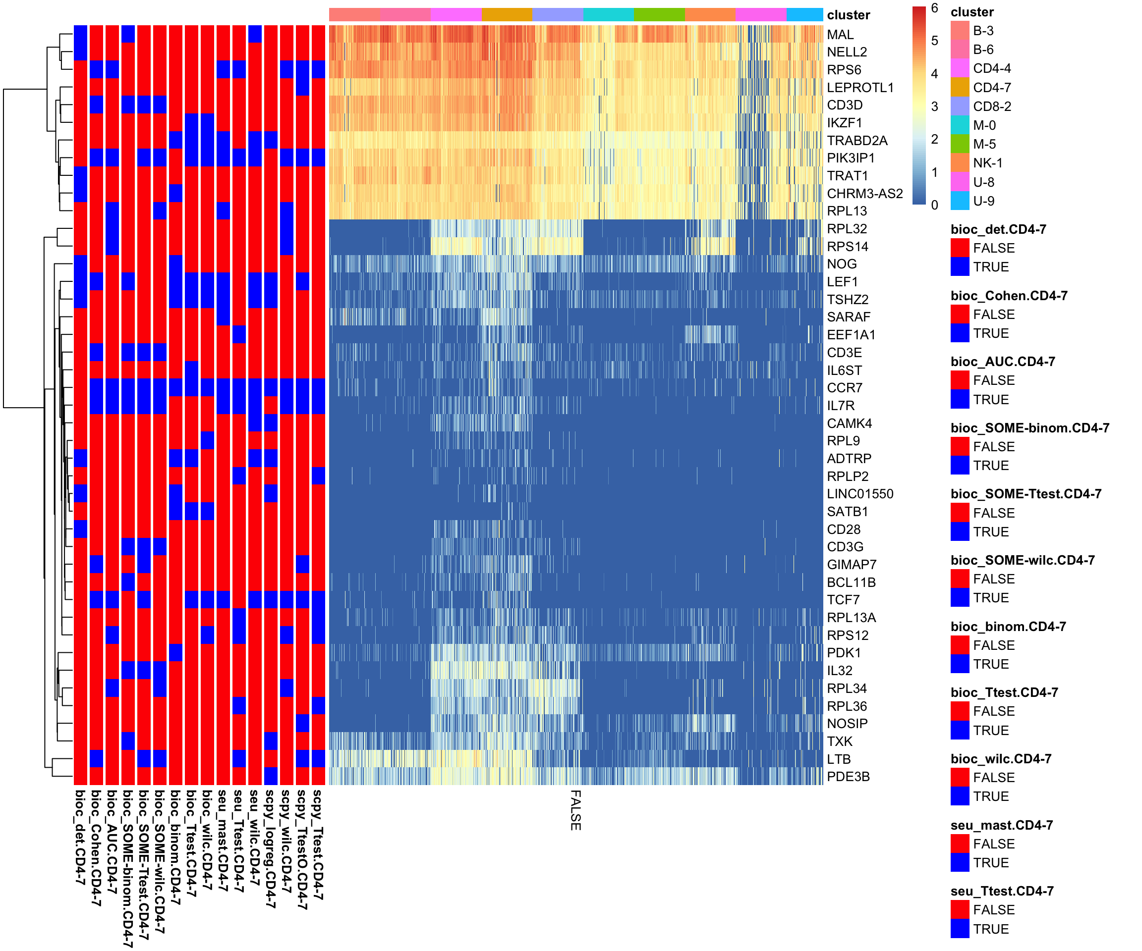

Not any clear signal for the CD4-7 cluster.

Quite a few ribosomal proteins among the DGEs.

The ribosomal proteins are high in all B/T cells and especially that cluster.

VlnPlot(all.sub, "percent_ribo", group.by = "cluster")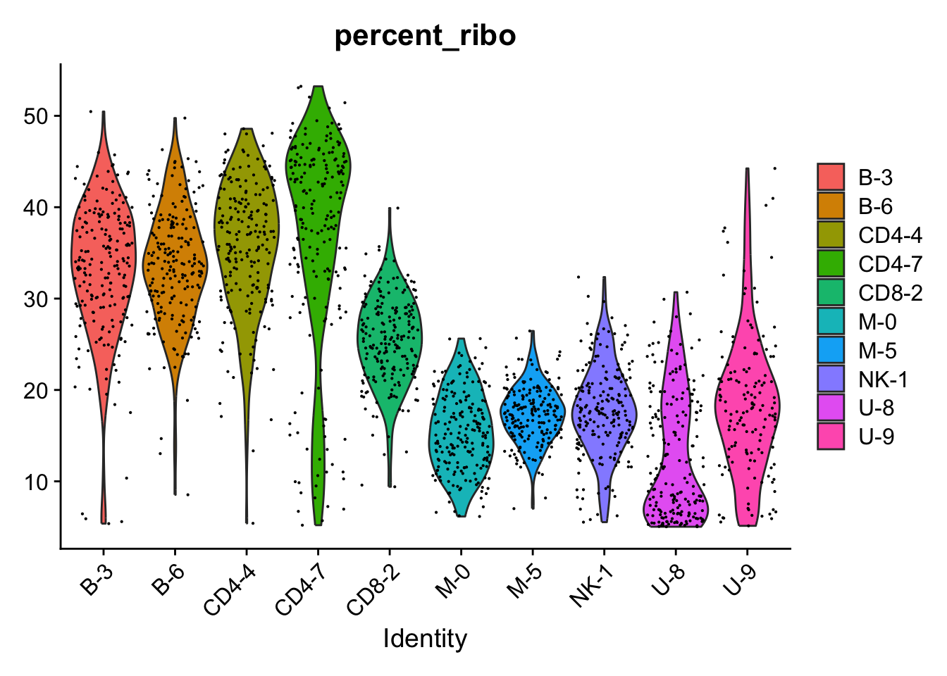

7.0.2 B-3

Same but for a B-cell cluster, take “B-3”

clust = "B-3"
sel = which(annot.tests$Cluster == clust)
topG = lapply(all.rank[sel], function(x) x[1:10])

gene_overlap_heatmap(topG)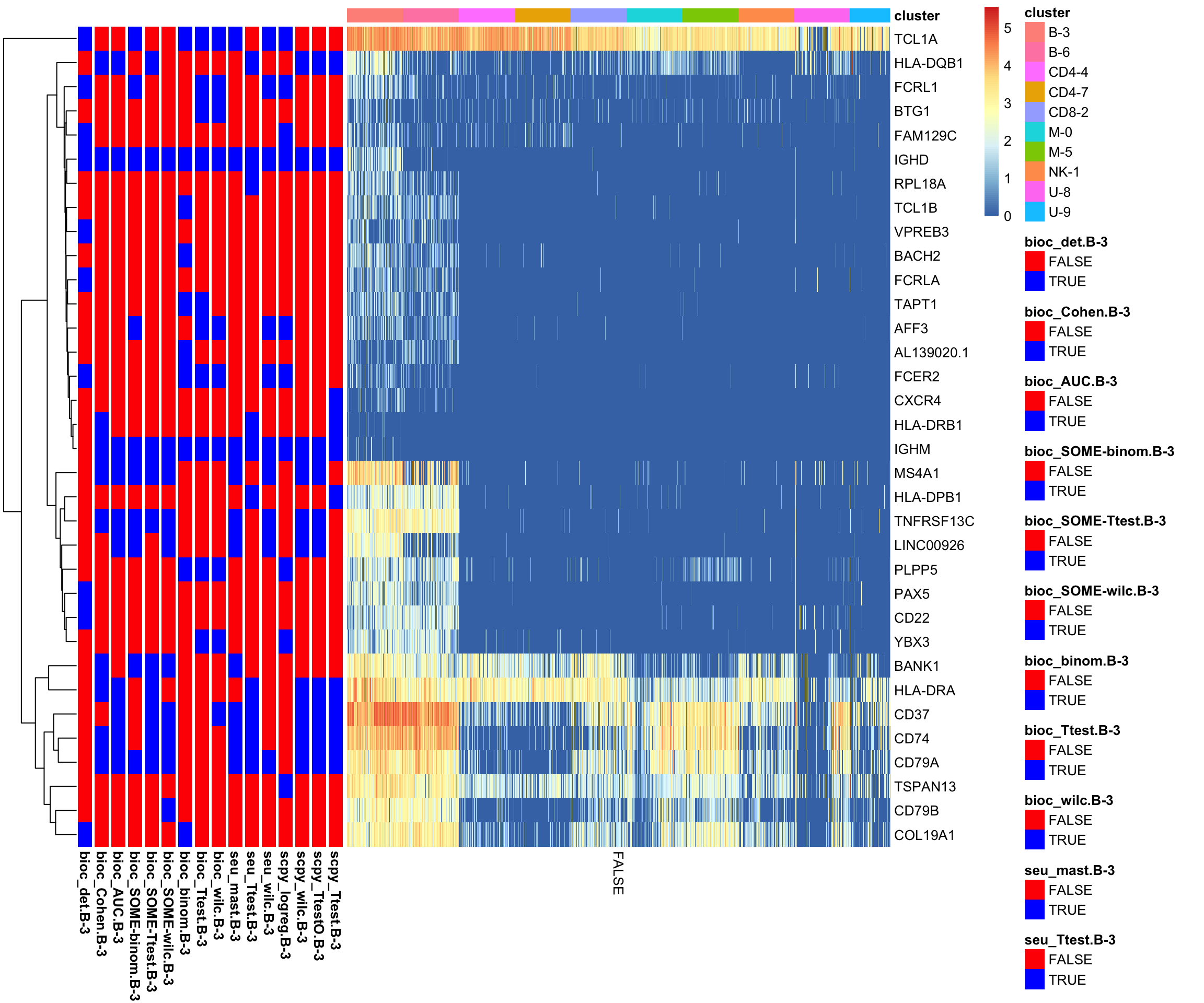

A few more clear markers.

8 Session info

Click here

sessionInfo()

R version 4.3.3 (2024-02-29)
Platform: x86_64-apple-darwin13.4.0 (64-bit)
Running under: macOS Big Sur ... 10.16

Matrix products: default
BLAS/LAPACK: /Users/asabjor/miniconda3/envs/seurat5_u/lib/libopenblasp-r0.3.28.dylib;  LAPACK version 3.12.0

locale:
[1] sv_SE.UTF-8/sv_SE.UTF-8/sv_SE.UTF-8/C/sv_SE.UTF-8/sv_SE.UTF-8

time zone: Europe/Stockholm
tzcode source: system (macOS)

attached base packages:
[1] grid      stats4    stats     graphics  grDevices utils     datasets 
[8] methods   base     

other attached packages:
 [1] pheatmap_1.0.12             ComplexHeatmap_2.18.0      
 [3] zellkonverter_1.12.1        basilisk.utils_1.14.1      
 [5] basilisk_1.14.1             scran_1.30.0               
 [7] scuttle_1.12.0              SingleCellExperiment_1.24.0
 [9] SummarizedExperiment_1.32.0 Biobase_2.62.0             
[11] GenomicRanges_1.54.1        GenomeInfoDb_1.38.1        
[13] IRanges_2.36.0              S4Vectors_0.40.2           
[15] BiocGenerics_0.48.1         MatrixGenerics_1.14.0      
[17] matrixStats_1.5.0           dplyr_1.1.4                
[19] patchwork_1.3.0             ggplot2_3.5.1              
[21] Matrix_1.6-5                Seurat_5.1.0               
[23] SeuratObject_5.0.2          sp_2.1-4                   

loaded via a namespace (and not attached):
  [1] RcppAnnoy_0.0.22          splines_4.3.3            
  [3] later_1.4.1               bitops_1.0-9             
  [5] filelock_1.0.3            tibble_3.2.1             
  [7] polyclip_1.10-7           fastDummies_1.7.4        
  [9] lifecycle_1.0.4           doParallel_1.0.17        
 [11] edgeR_4.0.16              globals_0.16.3           
 [13] lattice_0.22-6            MASS_7.3-60.0.1          
 [15] magrittr_2.0.3            limma_3.58.1             
 [17] plotly_4.10.4             rmarkdown_2.29           
 [19] remotes_2.5.0             yaml_2.3.10              
 [21] metapod_1.10.0            httpuv_1.6.15            
 [23] sctransform_0.4.1         spam_2.11-0              
 [25] sessioninfo_1.2.2         pkgbuild_1.4.5           
 [27] spatstat.sparse_3.1-0     reticulate_1.40.0        
 [29] cowplot_1.1.3             pbapply_1.7-2            
 [31] RColorBrewer_1.1-3        pkgload_1.4.0            
 [33] abind_1.4-5               zlibbioc_1.48.0          
 [35] Rtsne_0.17                purrr_1.0.2              
 [37] RCurl_1.98-1.16           circlize_0.4.16          
 [39] GenomeInfoDbData_1.2.11   ggrepel_0.9.6            
 [41] irlba_2.3.5.1             listenv_0.9.1            
 [43] spatstat.utils_3.1-2      goftest_1.2-3            
 [45] RSpectra_0.16-2           spatstat.random_3.3-2    
 [47] dqrng_0.3.2               fitdistrplus_1.2-2       
 [49] parallelly_1.41.0         DelayedMatrixStats_1.24.0
 [51] leiden_0.4.3.1            codetools_0.2-20         
 [53] DelayedArray_0.28.0       shape_1.4.6.1            
 [55] tidyselect_1.2.1          farver_2.1.2             
 [57] ScaledMatrix_1.10.0       spatstat.explore_3.3-4   
 [59] jsonlite_1.8.9            GetoptLong_1.0.5         
 [61] BiocNeighbors_1.20.0      ellipsis_0.3.2           
 [63] progressr_0.15.1          iterators_1.0.14         
 [65] ggridges_0.5.6            survival_3.8-3           
 [67] foreach_1.5.2             tools_4.3.3              
 [69] ica_1.0-3                 Rcpp_1.0.13-1            
 [71] glue_1.8.0                gridExtra_2.3            
 [73] SparseArray_1.2.2         xfun_0.50                
 [75] usethis_3.1.0             withr_3.0.2              
 [77] fastmap_1.2.0             bluster_1.12.0           
 [79] digest_0.6.37             rsvd_1.0.5               
 [81] R6_2.5.1                  mime_0.12                
 [83] colorspace_2.1-1          scattermore_1.2          
 [85] tensor_1.5                spatstat.data_3.1-4      
 [87] tidyr_1.3.1               generics_0.1.3           
 [89] data.table_1.15.4         httr_1.4.7               
 [91] htmlwidgets_1.6.4         S4Arrays_1.2.0           
 [93] uwot_0.1.16               pkgconfig_2.0.3          
 [95] gtable_0.3.6              lmtest_0.9-40            
 [97] XVector_0.42.0            htmltools_0.5.8.1        
 [99] profvis_0.4.0             dotCall64_1.2            
[101] clue_0.3-66               scales_1.3.0             
[103] png_0.1-8                 spatstat.univar_3.1-1    
[105] knitr_1.49                rjson_0.2.23             
[107] reshape2_1.4.4            curl_6.0.1               
[109] nlme_3.1-165              cachem_1.1.0             
[111] GlobalOptions_0.1.2       zoo_1.8-12               
[113] stringr_1.5.1             KernSmooth_2.23-26       
[115] vipor_0.4.7               parallel_4.3.3           
[117] miniUI_0.1.1.1            ggrastr_1.0.2            
[119] pillar_1.10.1             vctrs_0.6.5              
[121] RANN_2.6.2                urlchecker_1.0.1         
[123] promises_1.3.2            BiocSingular_1.18.0      
[125] beachmat_2.18.0           xtable_1.8-4             
[127] cluster_2.1.8             beeswarm_0.4.0           
[129] evaluate_1.0.1            cli_3.6.3                
[131] locfit_1.5-9.10           compiler_4.3.3           
[133] rlang_1.1.4               crayon_1.5.3             
[135] future.apply_1.11.2       labeling_0.4.3           
[137] ggbeeswarm_0.7.2          fs_1.6.5                 
[139] plyr_1.8.9                stringi_1.8.4            
[141] viridisLite_0.4.2         deldir_2.0-4             
[143] BiocParallel_1.36.0       munsell_0.5.1            
[145] lazyeval_0.2.2            devtools_2.4.5           
[147] spatstat.geom_3.3-4       dir.expiry_1.10.0        
[149] RcppHNSW_0.6.0            sparseMatrixStats_1.14.0 
[151] future_1.34.0             statmod_1.5.0            
[153] shiny_1.10.0              ROCR_1.0-11              
[155] memoise_2.0.1             igraph_2.0.3