suppressPackageStartupMessages({
    library(scater)
    library(scran)
    library(dplyr)
    library(patchwork)
    library(ggplot2)
    library(pheatmap)
    library(scPred)
    library(scmap)
    library(SingleR)
})
Note
Code chunks run R commands unless otherwise specified.
Celltype prediction can either be performed on indiviudal cells where each cell gets a predicted celltype label, or on the level of clusters. All methods are based on similarity to other datasets, single cell or sorted bulk RNAseq, or uses known marker genes for each cell type.
Ideally celltype predictions should be run on each sample separately and not using the integrated data. In this case we will select one sample from the Covid data, ctrl_13 and predict celltype by cell on that sample.
Some methods will predict a celltype to each cell based on what it is most similar to, even if that celltype is not included in the reference. Other methods include an uncertainty so that cells with low similarity scores will be unclassified.
There are multiple different methods to predict celltypes, here we will just cover a few of those.
We will use a reference PBMC dataset from the scPred package which is provided as a Seurat object with counts. And we will test classification based on the scPred and scMap methods. Finally we will use gene set enrichment predict celltype based on the DEGs of each cluster.
1 Read data
First, lets load required libraries
Let’s read in the saved Covid-19 data object from the clustering step.
# download pre-computed data if missing or long compute
fetch_data <- TRUE

# url for source and intermediate data
path_data <- "https://nextcloud.dc.scilifelab.se/public.php/webdav"
curl_upass <- "-u zbC5fr2LbEZ9rSE:scRNAseq2025"

path_file <- "data/covid/results/bioc_covid_qc_dr_int_cl.rds"
if (!dir.exists(dirname(path_file))) dir.create(dirname(path_file), recursive = TRUE)
if (fetch_data && !file.exists(path_file)) download.file(url = file.path(path_data, "covid/results_bioc/bioc_covid_qc_dr_int_cl.rds"), destfile = path_file, method = "curl", extra = curl_upass)

alldata <- readRDS(path_file)
Let’s read in the saved Covid-19 data object from the clustering step.
ctrl.sce <- alldata[, alldata$sample == "ctrl.13"]

# remove all old dimensionality reductions as they will mess up the analysis further down
reducedDims(ctrl.sce) <- NULL
2 Reference data
Load the reference dataset with annotated labels that is provided by the scPred package, it is a subsampled set of cells from human PBMCs.
reference <- scPred::pbmc_1
reference
An object of class Seurat
32838 features across 3500 samples within 1 assay
Active assay: RNA (32838 features, 0 variable features)
2 layers present: counts, dataConvert to a SCE object.
ref.sce <- Seurat::as.SingleCellExperiment(reference)Rerun analysis pipeline. Run normalization, feature selection and dimensionality reduction
# Normalize
ref.sce <- computeSumFactors(ref.sce)
ref.sce <- logNormCounts(ref.sce)

# Variable genes
var.out <- modelGeneVar(ref.sce, method = "loess")
hvg.ref <- getTopHVGs(var.out, n = 1000)

# Dim reduction
ref.sce <- runPCA(ref.sce,
    exprs_values = "logcounts", scale = T,
    ncomponents = 30, subset_row = hvg.ref
)
ref.sce <- runUMAP(ref.sce, dimred = "PCA")plotReducedDim(ref.sce, dimred = "UMAP", colour_by = "cell_type")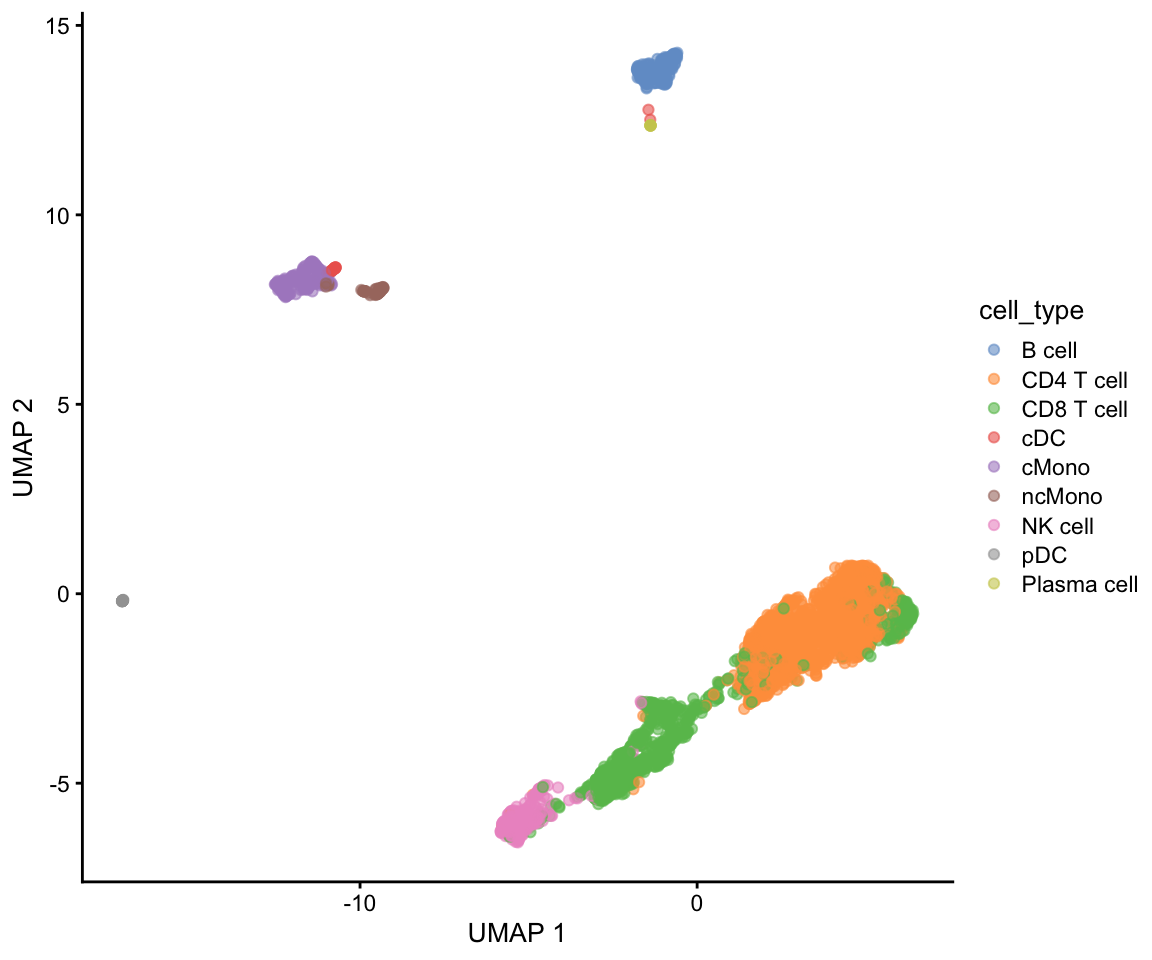
Run all steps of the analysis for the ctrl sample as well. Use the clustering from the integration lab with resolution 0.5.
# Normalize
ctrl.sce <- computeSumFactors(ctrl.sce)
ctrl.sce <- logNormCounts(ctrl.sce)

# Variable genes
var.out <- modelGeneVar(ctrl.sce, method = "loess")
hvg.ctrl <- getTopHVGs(var.out, n = 1000)

# Dim reduction
ctrl.sce <- runPCA(ctrl.sce, exprs_values = "logcounts", scale = T, ncomponents = 30, subset_row = hvg.ctrl)
ctrl.sce <- runUMAP(ctrl.sce, dimred = "PCA")plotReducedDim(ctrl.sce, dimred = "UMAP", colour_by = "leiden_k20")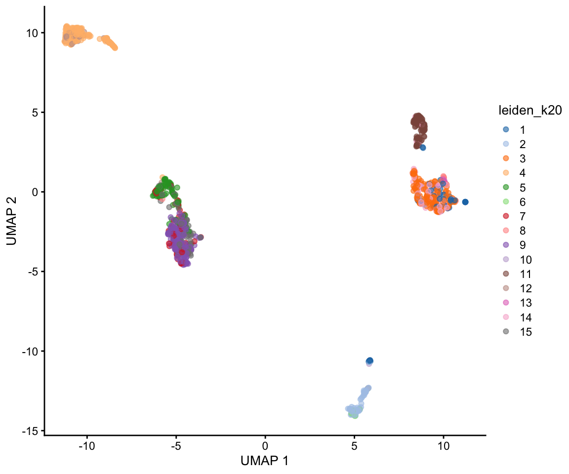
3 scMap
The scMap package is one method for projecting cells from a scRNA-seq experiment on to the cell-types or individual cells identified in a different experiment. It can be run on different levels, either projecting by cluster or by single cell, here we will try out both.
For scmap cell type labels must be stored in the cell_type1 column of the colData slots, and gene ids that are consistent across both datasets must be stored in the feature_symbol column of the rowData slots.
3.1 scMap cluster
# add in slot cell_type1
ref.sce$cell_type1 <- ref.sce$cell_type
# create a rowData slot with feature_symbol
rd <- data.frame(feature_symbol = rownames(ref.sce))
rownames(rd) <- rownames(ref.sce)
rowData(ref.sce) <- rd

# same for the ctrl dataset
# create a rowData slot with feature_symbol
rd <- data.frame(feature_symbol = rownames(ctrl.sce))
rownames(rd) <- rownames(ctrl.sce)
rowData(ctrl.sce) <- rd
Then we can select variable features in both datasets.
# select features
counts(ctrl.sce) <- as.matrix(counts(ctrl.sce))
logcounts(ctrl.sce) <- as.matrix(logcounts(ctrl.sce))
ctrl.sce <- selectFeatures(ctrl.sce, suppress_plot = TRUE)

counts(ref.sce) <- as.matrix(counts(ref.sce))
logcounts(ref.sce) <- as.matrix(logcounts(ref.sce))
ref.sce <- selectFeatures(ref.sce, suppress_plot = TRUE)
Then we need to index the reference dataset by cluster, default is the clusters in cell_type1.
ref.sce <- indexCluster(ref.sce)Now we project the Covid-19 dataset onto that index.
project_cluster <- scmapCluster(
    projection = ctrl.sce,
    index_list = list(
        ref = metadata(ref.sce)$scmap_cluster_index
    )
)

# projected labels
table(project_cluster$scmap_cluster_labs)
     B cell  CD4 T cell  CD8 T cell         cDC       cMono      ncMono
         72         109         113          31         201         137
    NK cell         pDC Plasma cell  unassigned
        281           2           1         156
Then add the predictions to metadata and plot UMAP.
# add in predictions
ctrl.sce$scmap_cluster <- project_cluster$scmap_cluster_labs

plotReducedDim(ctrl.sce, dimred = "UMAP", colour_by = "scmap_cluster")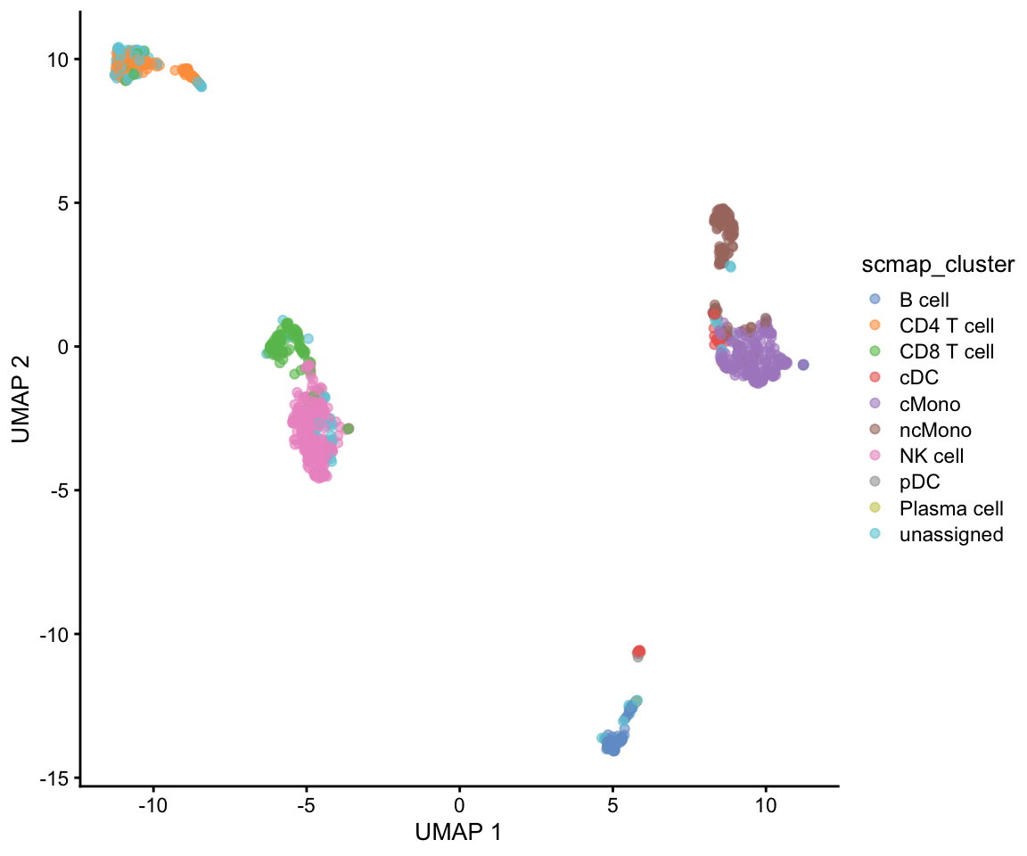
4 scMap cell
We can instead index the refernce data based on each single cell and project our data onto the closest neighbor in that dataset.
ref.sce <- indexCell(ref.sce)Again we need to index the reference dataset.
project_cell <- scmapCell(
    projection = ctrl.sce,
    index_list = list(
        ref = metadata(ref.sce)$scmap_cell_index
    )
)
We now get a table with index for the 5 nearest neigbors in the reference dataset for each cell in our dataset. We will select the celltype of the closest neighbor and assign it to the data.
cell_type_pred <- colData(ref.sce)$cell_type1[project_cell$ref[[1]][1, ]]
table(cell_type_pred)
cell_type_pred
B cell CD4 T cell CD8 T cell cDC cMono ncMono NK cell
95 168 247 46 217 132 197
pDC
1 Then add the predictions to metadata and plot umap.
# add in predictions
ctrl.sce$scmap_cell <- cell_type_pred

plotReducedDim(ctrl.sce, dimred = "UMAP", colour_by = "scmap_cell")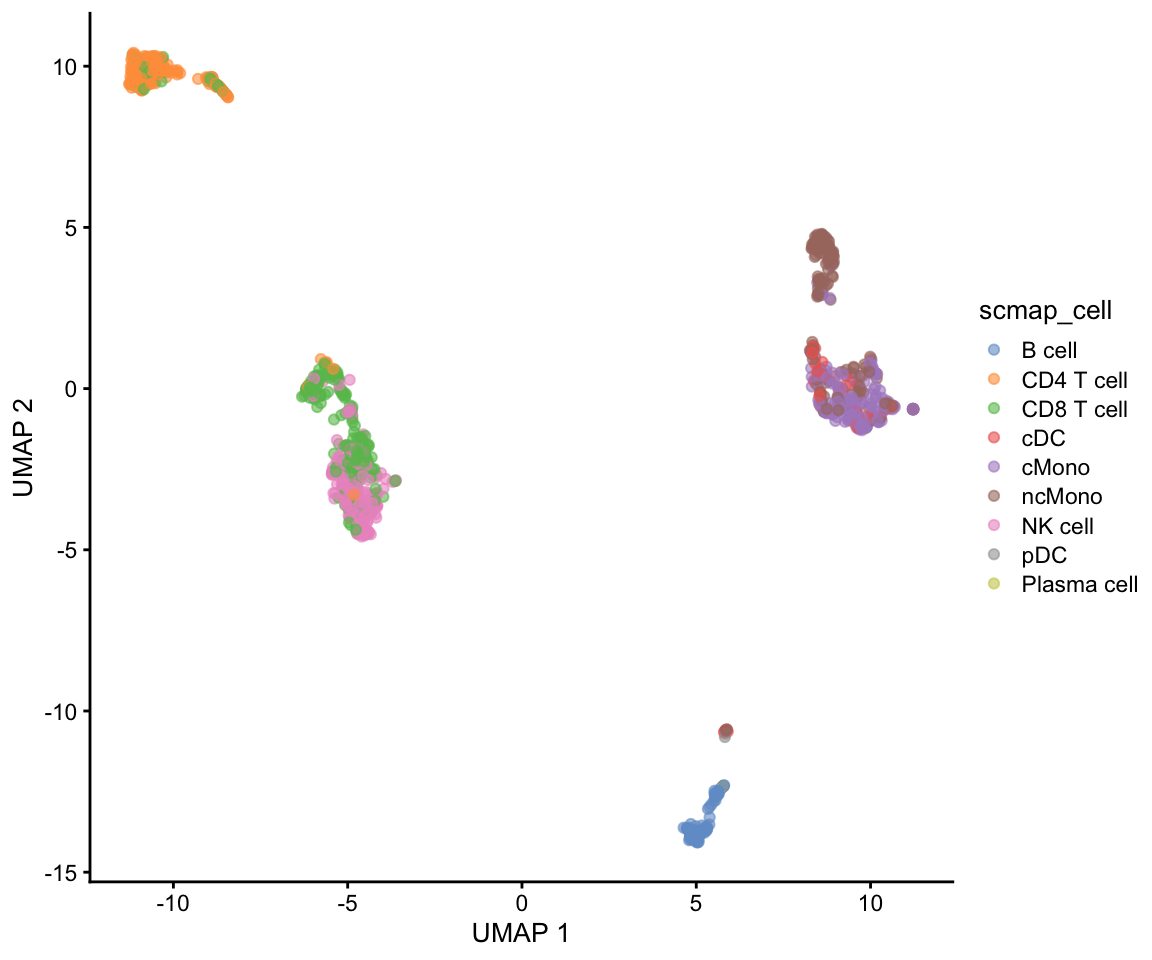
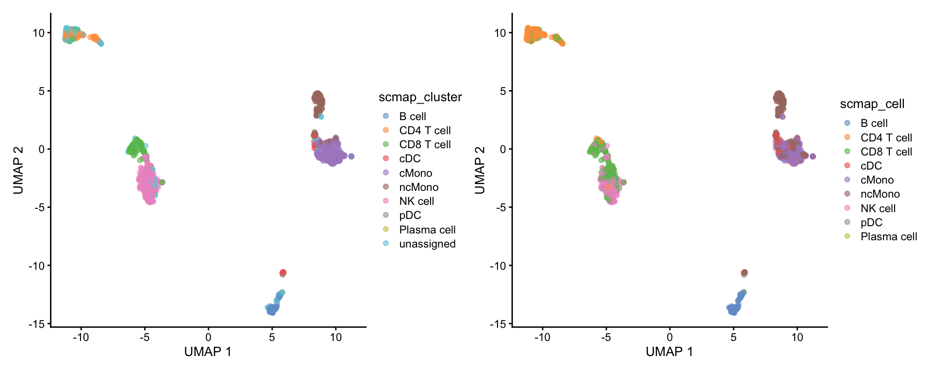
Plot both:
wrap_plots(
    plotReducedDim(ctrl.sce, dimred = "UMAP", colour_by = "scmap_cluster"),
    plotReducedDim(ctrl.sce, dimred = "UMAP", colour_by = "scmap_cell"),
    ncol = 2
)
5 SinlgeR
SingleR is performs unbiased cell type recognition from single-cell RNA sequencing data, by leveraging reference transcriptomic datasets of pure cell types to infer the cell of origin of each single cell independently.
There are multiple datasets included in the celldex package that can be used for celltype prediction, here we will test two different ones, the DatabaseImmuneCellExpressionData and the HumanPrimaryCellAtlasData. In addition we will use the same reference dataset that we used for label transfer above but using SingleR instead.
5.1 Immune cell reference
immune = celldex::DatabaseImmuneCellExpressionData()
singler.immune <- SingleR(test = ctrl.sce, ref = immune, assay.type.test=1,
    labels = immune$label.main)

head(singler.immune)
DataFrame with 6 rows and 4 columns
scores labels delta.next
<matrix> <character> <numeric>
AGGTCATGTGCGAACA-13 0.0679680:0.0760411:0.186694:... T cells, CD4+ 0.1375513
CCTATCGGTCCCTCAT-13 0.0027079:0.0960641:0.386088:... NK cells 0.1490740
TCCTCCCTCGTTCATT-13 0.0361115:0.1067465:0.394579:... NK cells 0.1220681
CAACCAATCATCTATC-13 0.0342030:0.1345967:0.402377:... NK cells 0.1513308
TACGGTATCGGATTAC-13 -0.0131813:0.0717678:0.283882:... NK cells 0.0620657
AATAGAGAGTTCGGTT-13 0.0841091:0.1367749:0.273738:... T cells, CD4+ 0.0660296
pruned.labels
<character>
AGGTCATGTGCGAACA-13 T cells, CD4+
CCTATCGGTCCCTCAT-13 NK cells
TCCTCCCTCGTTCATT-13 NK cells
CAACCAATCATCTATC-13 NK cells
TACGGTATCGGATTAC-13 NK cells
AATAGAGAGTTCGGTT-13 T cells, CD4+5.2 HPCA reference
hpca <- HumanPrimaryCellAtlasData()
singler.hpca <- SingleR(test = ctrl.sce, ref = hpca, assay.type.test=1,
    labels = hpca$label.main)

head(singler.hpca)
DataFrame with 6 rows and 4 columns
scores labels delta.next
<matrix> <character> <numeric>
AGGTCATGTGCGAACA-13 0.141378:0.310009:0.275987:... T_cells 0.4918992
CCTATCGGTCCCTCAT-13 0.145926:0.300045:0.277827:... NK_cell 0.3241970
TCCTCCCTCGTTCATT-13 0.132119:0.311754:0.274127:... NK_cell 0.0640608
CAACCAATCATCTATC-13 0.157184:0.302219:0.284496:... NK_cell 0.2012408
TACGGTATCGGATTAC-13 0.125120:0.283118:0.250322:... T_cells 0.1545913
AATAGAGAGTTCGGTT-13 0.191441:0.374422:0.329988:... T_cells 0.5063484
pruned.labels
<character>
AGGTCATGTGCGAACA-13 T_cells
CCTATCGGTCCCTCAT-13 NK_cell
TCCTCCCTCGTTCATT-13 NK_cell
CAACCAATCATCTATC-13 NK_cell
TACGGTATCGGATTAC-13 T_cells
AATAGAGAGTTCGGTT-13 T_cells5.3 With own reference data
singler.ref <- SingleR(test=ctrl.sce, ref=ref.sce, labels=ref.sce$cell_type, de.method="wilcox")
head(singler.ref)
DataFrame with 6 rows and 4 columns
scores labels delta.next
<matrix> <character> <numeric>
AGGTCATGTGCGAACA-13 0.741719:0.840093:0.805977:... CD4 T cell 0.0423204
CCTATCGGTCCCTCAT-13 0.649491:0.736753:0.815987:... NK cell 0.0451715
TCCTCCCTCGTTCATT-13 0.669603:0.731356:0.823308:... NK cell 0.0865526
CAACCAATCATCTATC-13 0.649948:0.721639:0.801202:... CD8 T cell 0.0740195
TACGGTATCGGATTAC-13 0.708827:0.776244:0.808044:... CD8 T cell 0.0905218
AATAGAGAGTTCGGTT-13 0.729010:0.847462:0.816299:... CD4 T cell 0.0409309
pruned.labels
<character>
AGGTCATGTGCGAACA-13 CD4 T cell
CCTATCGGTCCCTCAT-13 NK cell
TCCTCCCTCGTTCATT-13 NK cell
CAACCAATCATCTATC-13 CD8 T cell
TACGGTATCGGATTAC-13 CD8 T cell
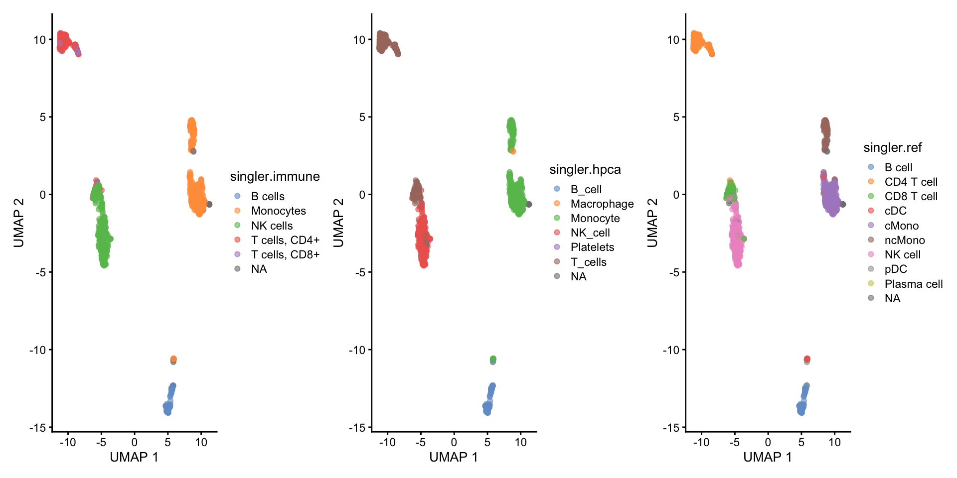
AATAGAGAGTTCGGTT-13 CD4 T cellCompare results:
ctrl.sce$singler.immune = singler.immune$pruned.labels
ctrl.sce$singler.hpca = singler.hpca$pruned.labels
ctrl.sce$singler.ref = singler.ref$pruned.labels

wrap_plots(
    plotReducedDim(ctrl.sce, dimred = "UMAP", colour_by = "singler.immune"),
    plotReducedDim(ctrl.sce, dimred = "UMAP", colour_by = "singler.hpca"),
    plotReducedDim(ctrl.sce, dimred = "UMAP", colour_by = "singler.ref"),
    ncol = 3
)
6 Compare results
Now we will compare the output of the two methods using the convenient function in scPred crossTab() that prints the overlap between two metadata slots.
table(ctrl.sce$scmap_cell, ctrl.sce$singler.hpca)
             B_cell Macrophage Monocyte NK_cell Platelets T_cells
  B cell         94          0        0       0         0       0
  CD4 T cell      0          0        0      11         0     155
  CD8 T cell      0          0        0     109         0     131
  cDC             0          0       42       0         0       0
  cMono           0          0      204       0         0       0
  ncMono          4          2      124       0         1       0
  NK cell         0          0        0     189         0       3
  pDC             1          0        0       0         0       0
Or plot onto umap:
wrap_plots(
    plotReducedDim(ctrl.sce, dimred = "UMAP", colour_by = "scmap_cluster"),
    plotReducedDim(ctrl.sce, dimred = "UMAP", colour_by = "scmap_cell"),
    plotReducedDim(ctrl.sce, dimred = "UMAP", colour_by = "singler.immune"),
    plotReducedDim(ctrl.sce, dimred = "UMAP", colour_by = "singler.hpca"),
    plotReducedDim(ctrl.sce, dimred = "UMAP", colour_by = "singler.ref"),
    ncol = 3
)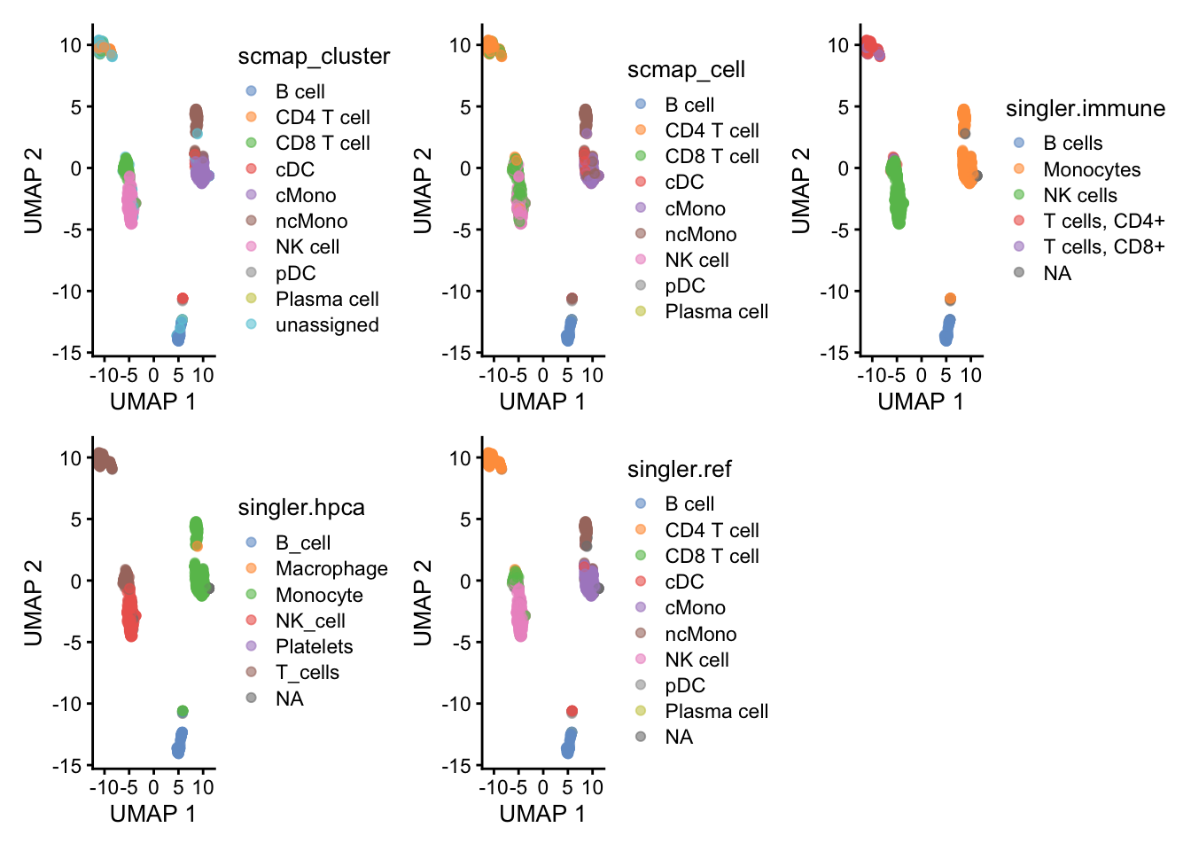
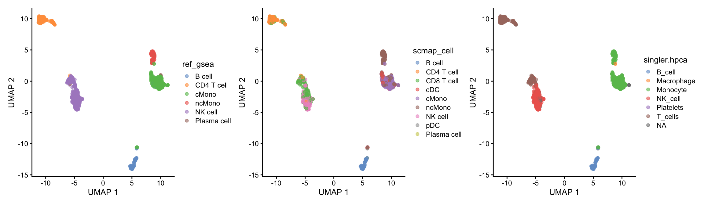
As you can see, the methods using the same reference all have similar results. While for instance singleR with different references give quite different predictions. This really shows that a relevant reference is the key in having reliable celltype predictions rather than the method used.
7 GSEA with celltype markers
Another option, where celltype can be classified on cluster level is to use gene set enrichment among the DEGs with known markers for different celltypes. Similar to how we did functional enrichment for the DEGs in the differential expression exercise. There are some resources for celltype gene sets that can be used. Such as CellMarker, PanglaoDB or celltype gene sets at MSigDB. We can also look at overlap between DEGs in a reference dataset and the dataset you are analyzing.
7.1 DEG overlap
First, lets extract top DEGs for our Covid-19 dataset and the reference dataset. When we run differential expression for our dataset, we want to report as many genes as possible, hence we set the cutoffs quite lenient.
# run differential expression in our dataset, using clustering at resolution 0.3
DGE_list <- scran::findMarkers(
    x = alldata,
    groups = as.character(alldata$leiden_k20),
    pval.type = "all",
    min.prop = 0
)
# Compute differential gene expression in reference dataset (that has cell annotation)
ref_DGE <- scran::findMarkers(
x = ref.sce,
groups = as.character(ref.sce$cell_type),
pval.type = "all",
direction = "up"
)
# Identify the top cell marker genes in reference dataset
# select top 50 with hihgest foldchange among top 100 signifcant genes.
ref_list <- lapply(ref_DGE, function(x) {
x$logFC <- rowSums(as.matrix(x[, grep("logFC", colnames(x))]))
x %>%
as.data.frame() %>%
filter(p.value < 0.01) %>%
top_n(-100, p.value) %>%
top_n(50, logFC) %>%
rownames()
})
unlist(lapply(ref_list, length)) B cell CD4 T cell CD8 T cell cDC cMono ncMono
50 50 19 17 50 50
NK cell pDC Plasma cell
50 50 24 Now we can run GSEA for the DEGs from our dataset and check for enrichment of top DEGs in the reference dataset.
suppressPackageStartupMessages(library(fgsea))

# run fgsea for each of the clusters in the list
res <- lapply(DGE_list, function(x) {
    x$logFC <- rowSums(as.matrix(x[, grep("logFC", colnames(x))]))
    gene_rank <- setNames(x$logFC, rownames(x))
    fgseaRes <- fgsea(pathways = ref_list, stats = gene_rank, nperm = 10000)
    return(fgseaRes)
})
names(res) <- names(DGE_list)

# You can filter and resort the table based on ES, NES or pvalue
res <- lapply(res, function(x) {
    x[x$pval < 0.1, ]
})
res <- lapply(res, function(x) {
    x[x$size > 2, ]
})
res <- lapply(res, function(x) {
    x[order(x$NES, decreasing = T), ]
})
res
$`1`
pathway pval padj ES NES nMoreExtreme size
<char> <num> <num> <num> <num> <num> <int>
1: NK cell 0.0474127557 0.085342960 -0.6730341 -1.304095 393 49
2: Plasma cell 0.0098219767 0.022099448 -0.7888373 -1.404130 79 24
3: cDC 0.0039472061 0.011841618 -0.8473729 -1.449569 31 17
4: B cell 0.0003613152 0.001625918 -0.7948789 -1.532491 2 47
5: CD4 T cell 0.0001201634 0.001081471 -0.9076362 -1.763345 0 50
leadingEdge
<list>
1: ITGB2, N....
2: PPIB, SU....
3: HLA-DRB1....
4: RPS23, R....
5: RPS6, RP....
$`10`
pathway pval padj ES NES nMoreExtreme size
<char> <num> <num> <num> <num> <num> <int>
1: cMono 0.00010001 0.000450045 0.9408130 1.467697 0 47
2: ncMono 0.00010000 0.000450045 0.9111705 1.423095 0 49
3: cDC 0.03560231 0.053403459 0.8242284 1.235247 351 17
4: CD4 T cell 0.01250000 0.028125000 0.7654381 1.196170 124 50
5: pDC 0.02880288 0.051845185 0.7510573 1.171672 287 47
6: CD8 T cell 0.01041667 0.028125000 -0.9666325 -2.385116 0 18
leadingEdge
<list>
1: S100A9, ....
2: S100A11,....
3: HLA-DRA,....
4: RPS13, T....
5: CTSB, PL....
6: IL32, CC....
$`11`
pathway pval padj ES NES nMoreExtreme
<char> <num> <num> <num> <num> <num>
1: B cell 0.0625357265 0.0703526924 -0.6836964 -1.317659 546
2: CD4 T cell 0.0510527507 0.0656392509 -0.6851698 -1.330576 450
3: NK cell 0.0284673195 0.0427009793 -0.7082648 -1.371671 249
4: pDC 0.0078884189 0.0167474774 -0.7508872 -1.447153 68
5: cDC 0.0093041541 0.0167474774 -0.8571692 -1.463250 70
6: Plasma cell 0.0005011275 0.0015033826 -0.8856248 -1.578622 3
7: cMono 0.0001143249 0.0005144621 -0.8936173 -1.722231 0
8: ncMono 0.0001138693 0.0005144621 -0.9057447 -1.754124 0
size leadingEdge
<int> <list>
1: 47 FAU, RPS....
2: 50 RPS13, R....
3: 49 ITGB2, B....
4: 47 PLEK, NP....
5: 17 HLA-DRA,....
6: 24 RPL36AL,....
7: 47 LYZ, S10....
8: 49 FTH1, S1....
$`12`
pathway pval padj ES NES nMoreExtreme size
<char> <num> <num> <num> <num> <num> <int>
1: cDC 0.0005182018 0.00214490 0.9499077 1.630649 3 17
2: CD4 T cell 0.0005566069 0.00214490 0.8315386 1.596805 4 50
3: pDC 0.0544965239 0.09809374 0.7040968 1.346143 485 47
4: B cell 0.0953128504 0.12982081 0.6734264 1.287505 849 47
5: CD8 T cell 0.0008904720 0.00214490 -0.8818421 -1.909414 1 18
6: NK cell 0.0009532888 0.00214490 -0.7785027 -2.071824 0 49
leadingEdge
<list>
1: HLA-DRA,....
2: RPL5, RP....
3: PPP1R14B....
4: RPS23, R....
5: CCL5, IL....
6: NKG7, BI....
$`2`
pathway pval padj ES NES nMoreExtreme size
<char> <num> <num> <num> <num> <num> <int>
1: B cell 0.0001983733 0.0004557424 0.9679870 2.009014 0 47
2: CD4 T cell 0.0001964637 0.0004557424 0.8820766 1.850463 0 50
3: cDC 0.0031243491 0.0046865236 0.9089562 1.611749 14 17
4: CD8 T cell 0.0036693704 0.0047177620 -0.8923493 -1.614725 18 18
5: cMono 0.0004031445 0.0007256601 -0.8362670 -1.774346 1 47
6: ncMono 0.0002025522 0.0004557424 -0.8849694 -1.888526 0 49
7: NK cell 0.0002025522 0.0004557424 -0.8875946 -1.894128 0 49
leadingEdge
<list>
1: MS4A1, C....
2: RPS29, R....
3: HLA-DRA,....
4: CCL5, IL....
5: LYZ, S10....
6: S100A4, ....
7: ITGB2, H....
$`3`
pathway pval padj ES NES nMoreExtreme
<char> <num> <num> <num> <num> <num>
1: cMono 0.0001190760 0.0005358419 0.9583409 1.782039 0
2: ncMono 0.0001184975 0.0005358419 0.9023835 1.683224 0
3: Plasma cell 0.0141185962 0.0181524808 -0.7509683 -1.590219 34
4: NK cell 0.0012795905 0.0019193858 -0.7386851 -1.791018 1
5: CD8 T cell 0.0003496503 0.0010489510 -0.9296700 -1.838145 0
6: B cell 0.0006234414 0.0011627907 -0.8317124 -2.004087 0
7: CD4 T cell 0.0006459948 0.0011627907 -0.8953192 -2.180214 0
size leadingEdge
<int> <list>
1: 47 S100A9, ....
2: 49 AIF1, S1....
3: 24 ISG20, P....
4: 49 GNLY, NK....
5: 18 IL32, CC....
6: 47 CXCR4, R....
7: 50 RPL3, RP....
$`4`
pathway pval padj ES NES nMoreExtreme size
<char> <num> <num> <num> <num> <num> <int>
1: CD4 T cell 0.0001808318 0.0006675567 0.9775430 2.019099 0 50
2: B cell 0.0027452416 0.0041178624 0.7829302 1.597888 14 47
3: pDC 0.0015425297 0.0027765535 -0.7838592 -1.680259 6 47
4: cDC 0.0008120179 0.0018270402 -0.9271115 -1.682592 3 17
5: cMono 0.0002203614 0.0006675567 -0.9154263 -1.962282 0 47
6: ncMono 0.0002225189 0.0006675567 -0.9350273 -2.015045 0 49
leadingEdge
<list>
1: IL7R, RP....
2: RPS5, RP....
3: PLEK, NP....
4: HLA-DRA,....
5: S100A9, ....
6: FCER1G, ....
$`5`
pathway pval padj ES NES nMoreExtreme
<char> <num> <num> <num> <num> <num>
1: NK cell 0.0001908761 0.0003779131 0.9534246 1.990389 0
2: CD4 T cell 0.0001915709 0.0003779131 0.8743701 1.829781 0
3: CD8 T cell 0.0002009646 0.0003779131 0.9620926 1.722598 0
4: Plasma cell 0.0739485748 0.0950767391 0.7540575 1.405239 370
5: cDC 0.0015879317 0.0023818976 -0.9128672 -1.639552 7
6: ncMono 0.0002099517 0.0003779131 -0.8774352 -1.878655 0
7: cMono 0.0002085506 0.0003779131 -0.9187853 -1.954299 0
size leadingEdge
<int> <list>
1: 49 NKG7, GN....
2: 50 RPS29, R....
3: 18 CCL5, IL....
4: 24 RPL36AL,....
5: 17 HLA-DRA,....
6: 49 FCER1G, ....
7: 47 S100A9, ....
$`6`
pathway pval padj ES NES nMoreExtreme
<char> <num> <num> <num> <num> <num>
1: cMono 0.0015649452 0.0028169014 0.9588064 2.255291 0
2: ncMono 0.0032000000 0.0048000000 0.7679881 1.815338 1
3: cDC 0.0384785984 0.0432884232 -0.7886041 -1.321383 346
4: CD8 T cell 0.0108467072 0.0139457665 -0.8256435 -1.389050 97
5: B cell 0.0004272135 0.0009612304 -0.7802534 -1.425878 3
6: NK cell 0.0001066439 0.0003271894 -0.8016664 -1.469451 0
7: Plasma cell 0.0001090631 0.0003271894 -0.8996256 -1.558065 0
8: CD4 T cell 0.0001065644 0.0003271894 -0.9203083 -1.689365 0
size leadingEdge
<int> <list>
1: 47 S100A9, ....
2: 49 AIF1, S1....
3: 17 HLA-DPA1....
4: 18 CCL5, IL....
5: 47 RPS5, RP....
6: 49 B2M, NKG....
7: 24 RPL36AL,....
8: 50 RPL3, RP....
$`7`
pathway pval padj ES NES nMoreExtreme size
<char> <num> <num> <num> <num> <num> <int>
1: NK cell 0.0002841716 0.001278772 0.9795593 2.108325 0 49
2: CD8 T cell 0.0029016091 0.004377208 0.9262395 1.719668 10 18
3: B cell 0.0035482876 0.004562084 -0.7866099 -1.586739 22 47
4: CD4 T cell 0.0029181385 0.004377208 -0.7804130 -1.589146 18 50
5: cDC 0.0014481094 0.003258246 -0.9146071 -1.593753 8 17
6: ncMono 0.0010797470 0.003239241 -0.8124991 -1.647792 6 49
7: cMono 0.0001542734 0.001278772 -0.9090987 -1.833822 0 47
leadingEdge
<list>
1: GNLY, NK....
2: CCL5, GZ....
3: RPS11, R....
4: TMEM123,....
5: HLA-DRA,....
6: COTL1, A....
7: S100A9, ....
$`8`
pathway pval padj ES NES nMoreExtreme
<char> <num> <num> <num> <num> <num>
1: Plasma cell 0.0013262599 0.0023872679 0.9401590 2.199892 0
2: cDC 0.0176490176 0.0264735265 -0.8172026 -1.377792 158
3: CD4 T cell 0.0010385294 0.0023366912 -0.7730462 -1.420728 9
4: NK cell 0.0006243496 0.0018730489 -0.7927600 -1.454472 5
5: cMono 0.0001041884 0.0004688477 -0.8921688 -1.632576 0
6: ncMono 0.0001040583 0.0004688477 -0.9199504 -1.687828 0
size leadingEdge
<int> <list>
1: 24 JCHAIN, ....
2: 17 HLA-DRB1....
3: 50 RPL38, R....
4: 49 ITGB2, H....
5: 47 S100A8, ....
6: 49 S100A4, ....
$`9`
pathway pval padj ES NES nMoreExtreme size
<char> <num> <num> <num> <num> <num> <int>
1: ncMono 0.0001140121 0.001026109 0.9763618 1.784597 0 49
2: cDC 0.0459984047 0.082797128 0.8377712 1.379493 345 17
3: Plasma cell 0.0863137816 0.129470672 -0.6440197 -1.377806 180 24
4: NK cell 0.0008123477 0.001870324 -0.7420783 -1.837291 0 49
5: CD8 T cell 0.0004078303 0.001835237 -0.9244331 -1.855656 0 18
6: CD4 T cell 0.0008312552 0.001870324 -0.8668681 -2.154953 0 50
leadingEdge
<list>
1: LST1, FC....
2: HLA-DPA1....
3: PEBP1, F....
4: NKG7, GN....
5: CCL5, IL....
6: LDHB, IL....Selecting top significant overlap per cluster, we can now rename the clusters according to the predicted labels. OBS! Be aware that if you have some clusters that have non-significant p-values for all the gene sets, the cluster label will not be very reliable. Also, the gene sets you are using may not cover all the celltypes you have in your dataset and hence predictions may just be the most similar celltype. Also, some of the clusters have very similar p-values to multiple celltypes, for instance the ncMono and cMono celltypes are equally good for some clusters.
new.cluster.ids <- unlist(lapply(res, function(x) {
as.data.frame(x)[1, 1]
}))
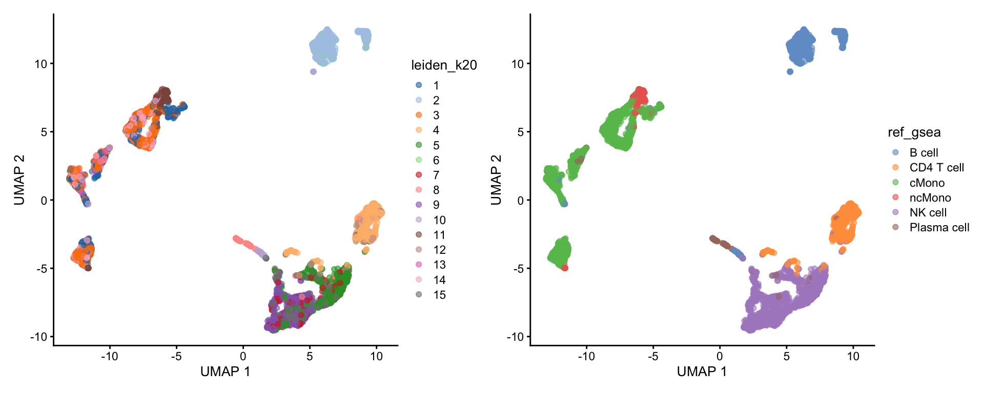
alldata$ref_gsea <- new.cluster.ids[as.character(alldata$leiden_k20)]
wrap_plots(
plotReducedDim(alldata, dimred = "UMAP", colour_by = "leiden_k20"),
plotReducedDim(alldata, dimred = "UMAP", colour_by = "ref_gsea"),
ncol = 2
)
Compare the results with the other celltype prediction methods in the ctrl_13 sample.
ctrl.sce$ref_gsea <- alldata$ref_gsea[alldata$sample == "ctrl.13"]

wrap_plots(
    plotReducedDim(ctrl.sce, dimred = "UMAP", colour_by = "ref_gsea"),
    plotReducedDim(ctrl.sce, dimred = "UMAP", colour_by = "scmap_cell"),
    plotReducedDim(ctrl.sce, dimred = "UMAP", colour_by = "singler.hpca"),
    ncol = 3
)
7.2 With annotated gene sets
We have downloaded the celltype gene lists from http://bio-bigdata.hrbmu.edu.cn/CellMarker/CellMarker_download.html and converted the excel file to a csv for you. Read in the gene lists and do some filtering.
path_file <- file.path("data/human_cell_markers.txt")
if (!file.exists(path_file)) download.file(file.path(path_data, "misc/cell_marker_human.csv"), destfile = path_file, method = "curl", extra = curl_upass)
markers <- read.delim("data/human_cell_markers.txt")
markers <- markers[markers$speciesType == "Human", ]
markers <- markers[markers$cancerType == "Normal", ]
# Filter by tissue (to reduce computational time and have tissue-specific classification)
# sort(unique(markers$tissueType))
# grep("blood",unique(markers$tissueType),value = T)
# markers <- markers [ markers$tissueType %in% c("Blood","Venous blood",
# "Serum","Plasma",
# "Spleen","Bone marrow","Lymph node"), ]
# remove strange characters etc.
celltype_list <- lapply(unique(markers$cellName), function(x) {
x <- paste(markers$geneSymbol[markers$cellName == x], sep = ",")
x <- gsub("[[]|[]]| |-", ",", x)
x <- unlist(strsplit(x, split = ","))
x <- unique(x[!x %in% c("", "NA", "family")])
x <- casefold(x, upper = T)
})
names(celltype_list) <- unique(markers$cellName)
# celltype_list <- lapply(celltype_list , function(x) {x[1:min(length(x),50)]} )
celltype_list <- celltype_list[unlist(lapply(celltype_list, length)) < 100]
celltype_list <- celltype_list[unlist(lapply(celltype_list, length)) > 5]# run fgsea for each of the clusters in the list
res <- lapply(DGE_list, function(x) {
x$logFC <- rowSums(as.matrix(x[, grep("logFC", colnames(x))]))
gene_rank <- setNames(x$logFC, rownames(x))
fgseaRes <- fgsea(pathways = celltype_list, stats = gene_rank, nperm = 10000)
return(fgseaRes)
})
names(res) <- names(DGE_list)
# You can filter and resort the table based on ES, NES or pvalue
res <- lapply(res, function(x) {
x[x$pval < 0.01, ]
})
res <- lapply(res, function(x) {
x[x$size > 5, ]
})
res <- lapply(res, function(x) {
x[order(x$NES, decreasing = T), ]
})
# show top 3 for each cluster.
lapply(res, head, 3)$`1`
pathway pval padj ES NES nMoreExtreme
<char> <num> <num> <num> <num> <num>
1: Megakaryocyte 0.0005482456 0.05153509 0.9246274 1.895872 0
2: Platelet 0.0017636684 0.11052322 0.7909662 1.797915 2
3: Embryonic stem cell 0.0082236842 0.24436945 0.8121999 1.665349 14
size leadingEdge
<int> <list>
1: 26 PPBP, PF....
2: 45 GP9, ITG....
3: 26 CD9, ITG....
$`10`
pathway pval padj ES NES
<char> <num> <num> <num> <num>
1: Neutrophil 0.0000999900 0.008155003 0.8918864 1.408530
2: Monocyte derived dendritic cell 0.0003036437 0.008155003 0.9324964 1.406936
3: Glial cell 0.0004124137 0.009406585 0.9479401 1.400298
nMoreExtreme size leadingEdge
<num> <int> <list>
1: 0 82 S100A9, ....
2: 2 18 S100A9, ....
3: 3 12 CD14, VI....
$`11`
pathway pval padj ES NES nMoreExtreme
<char> <num> <num> <num> <num> <num>
1: T helper2 (Th2) cell 0.0005534034 0.01733997 0.8544554 1.988856 0
2: CD4+ T cell 0.0005141388 0.01733997 0.8522778 1.941450 0
3: Naive CD8+ T cell 0.0016260163 0.04367015 0.6527521 1.836885 0
size leadingEdge
<int> <list>
1: 28 CCR7, CD....
2: 25 IL7R, LT....
3: 91 ATM, TCF....
$`12`
pathway pval padj ES NES
<char> <num> <num> <num> <num>
1: Morula cell (Blastomere) 0.0001051967 0.01977698 0.7866169 1.580081
2: FOXN4+ cell 0.0028790787 0.04920607 0.7447230 1.482096
3: Radial glial cell 0.0036215482 0.05237316 0.9638165 1.472593
nMoreExtreme size leadingEdge
<num> <int> <list>
1: 0 88 LDHA, RP....
2: 26 75 LYZ, ENO....
3: 23 7 VIM, TNC
$`2`
pathway pval padj ES NES
<char> <num> <num> <num> <num>
1: Follicular B cell 0.009543147 0.07974052 0.8609306 1.574668
2: Pyramidal cell 0.005240683 0.05795579 -0.9696824 -1.475255
3: CD4+CD25+ regulatory T cell 0.001940994 0.03649068 -0.9809077 -1.492333
nMoreExtreme size leadingEdge
<num> <int> <list>
1: 46 22 MS4A1, C....
2: 26 6 NRGN, CD3E
3: 9 6 CD3E, CD....
$`3`
pathway pval padj ES NES
<char> <num> <num> <num> <num>
1: Neutrophil 0.0001110001 0.007729945 0.9106943 1.771658
2: CD1C+_B dendritic cell 0.0001176886 0.007729945 0.9146942 1.717916
3: Stromal cell 0.0001233502 0.007729945 0.8852017 1.608791
nMoreExtreme size leadingEdge
<num> <int> <list>
1: 0 82 S100A9, ....
2: 0 54 S100A9, ....
3: 0 38 VIM, CD4....
$`4`
pathway pval padj ES NES nMoreExtreme
<char> <num> <num> <num> <num> <num>
1: Naive CD8+ T cell 0.0001723247 0.008795322 0.8487194 1.900408 0
2: Naive CD4+ T cell 0.0001915342 0.008795322 0.9111666 1.764006 0
3: CD4+ T cell 0.0003913894 0.012263536 0.9226665 1.703651 1
size leadingEdge
<int> <list>
1: 91 LDHB, PI....
2: 34 IL7R, RP....
3: 25 LTB, IL7....
$`5`
pathway pval padj ES
<char> <num> <num> <num>
1: CD4+ cytotoxic T cell 0.0001848429 0.006774775 0.8914605
2: Effector CD8+ memory T (Tem) cell 0.0001870907 0.006774775 0.8165710
3: Natural killer cell 0.0001853568 0.006774775 0.7977051
NES nMoreExtreme size leadingEdge
<num> <num> <int> <list>
1: 2.013200 0 86 NKG7, CC....
2: 1.821246 0 79 GNLY, GZ....
3: 1.795441 0 84 NKG7, GN....
$`6`
pathway pval padj ES NES
<char> <num> <num> <num> <num>
1: Neutrophil 0.002415459 0.1139394 0.9007177 2.310098
2: CD1C+_B dendritic cell 0.001727116 0.1139394 0.9326342 2.286423
3: Monocyte derived dendritic cell 0.003024194 0.1139394 0.9104408 1.908919
nMoreExtreme size leadingEdge
<num> <int> <list>
1: 0 82 S100A9, ....
2: 0 54 S100A9, ....
3: 2 18 S100A9, ....
$`7`
pathway pval padj ES NES
<char> <num> <num> <num> <num>
1: CD4+ cytotoxic T cell 0.0003015682 0.01140085 0.9435417 2.188179
2: Effector CD8+ memory T (Tem) cell 0.0003032141 0.01140085 0.9035783 2.073115
3: Natural killer cell 0.0003031222 0.01140085 0.8389683 1.940036
nMoreExtreme size leadingEdge
<num> <int> <list>
1: 0 86 GNLY, NK....
2: 0 79 GNLY, GZ....
3: 0 84 GNLY, NK....
$`8`
pathway pval padj ES NES
<char> <num> <num> <num> <num>
1: Megakaryocyte erythroid cell 0.008318961 0.03933770 -0.6843618 -1.293665
2: Naive CD8+ T cell 0.006377164 0.03330297 -0.6824089 -1.295030
3: Natural killer cell 0.006088898 0.03330297 -0.6906342 -1.305876
nMoreExtreme size leadingEdge
<num> <int> <list>
1: 81 83 PTPRC, C....
2: 62 91 AIF1, TO....
3: 59 84 PTPRC, I....
$`9`
pathway pval padj ES NES nMoreExtreme
<char> <num> <num> <num> <num> <num>
1: Mesenchymal cell 0.0002237136 0.04205817 0.8390045 1.567435 1
2: Stromal cell 0.0020332496 0.09556273 0.8473531 1.527840 16
3: Hemangioblast 0.0004689698 0.04408316 0.9863675 1.499066 2
size leadingEdge
<int> <list>
1: 61 COTL1, S....
2: 38 PECAM1, ....
3: 8 PECAM1, ....#CT_GSEA8:
new.cluster.ids <- unlist(lapply(res, function(x) {
as.data.frame(x)[1, 1]
}))
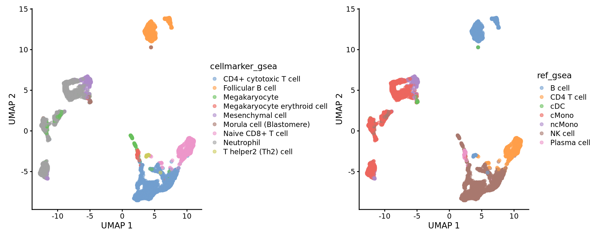
alldata$cellmarker_gsea <- new.cluster.ids[as.character(alldata$leiden_k20)]
wrap_plots(
plotReducedDim(alldata, dimred = "UMAP", colour_by = "cellmarker_gsea"),
plotReducedDim(alldata, dimred = "UMAP", colour_by = "ref_gsea"),
ncol = 2
)
Discuss
Do you think that the methods overlap well? Where do you see the most inconsistencies?
In this case we do not have any ground truth, and we cannot say which method performs best. You should keep in mind, that any celltype classification method is just a prediction, and you still need to use your common sense and knowledge of the biological system to judge if the results make sense.
Finally, lets save the data with predictions.
saveRDS(ctrl.sce, "data/covid/results/bioc_covid_qc_dr_int_cl_ct-ctrl13.rds")8 Session info
Click here
sessionInfo()R version 4.3.3 (2024-02-29)
Platform: x86_64-conda-linux-gnu (64-bit)
Running under: Ubuntu 20.04.6 LTS
Matrix products: default
BLAS/LAPACK: /usr/local/conda/envs/seurat/lib/libopenblasp-r0.3.28.so; LAPACK version 3.12.0
locale:
[1] LC_CTYPE=en_US.UTF-8 LC_NUMERIC=C
[3] LC_TIME=en_US.UTF-8 LC_COLLATE=en_US.UTF-8
[5] LC_MONETARY=en_US.UTF-8 LC_MESSAGES=en_US.UTF-8
[7] LC_PAPER=en_US.UTF-8 LC_NAME=C
[9] LC_ADDRESS=C LC_TELEPHONE=C
[11] LC_MEASUREMENT=en_US.UTF-8 LC_IDENTIFICATION=C
time zone: Etc/UTC
tzcode source: system (glibc)
attached base packages:
[1] stats4 stats graphics grDevices utils datasets methods
[8] base
other attached packages:
[1] fgsea_1.28.0 celldex_1.12.0
[3] Seurat_5.1.0 SeuratObject_5.0.2
[5] sp_2.2-0 SingleR_2.4.0
[7] scmap_1.24.0 scPred_1.9.2
[9] pheatmap_1.0.12 patchwork_1.3.0
[11] dplyr_1.1.4 scran_1.30.0
[13] scater_1.30.1 ggplot2_3.5.1
[15] scuttle_1.12.0 SingleCellExperiment_1.24.0
[17] SummarizedExperiment_1.32.0 Biobase_2.62.0
[19] GenomicRanges_1.54.1 GenomeInfoDb_1.38.1
[21] IRanges_2.36.0 S4Vectors_0.40.2
[23] BiocGenerics_0.48.1 MatrixGenerics_1.14.0
[25] matrixStats_1.5.0
loaded via a namespace (and not attached):
[1] spatstat.sparse_3.1-0 bitops_1.0-9
[3] lubridate_1.9.4 httr_1.4.7
[5] RColorBrewer_1.1-3 tools_4.3.3
[7] sctransform_0.4.1 R6_2.6.1
[9] lazyeval_0.2.2 uwot_0.2.2
[11] withr_3.0.2 gridExtra_2.3
[13] progressr_0.15.1 cli_3.6.4
[15] spatstat.explore_3.3-4 fastDummies_1.7.5
[17] labeling_0.4.3 spatstat.data_3.1-4
[19] randomForest_4.7-1.2 proxy_0.4-27
[21] ggridges_0.5.6 pbapply_1.7-2
[23] harmony_1.2.1 parallelly_1.42.0
[25] limma_3.58.1 RSQLite_2.3.9
[27] FNN_1.1.4.1 generics_0.1.3
[29] ica_1.0-3 spatstat.random_3.3-2
[31] Matrix_1.6-5 ggbeeswarm_0.7.2
[33] abind_1.4-5 lifecycle_1.0.4
[35] yaml_2.3.10 edgeR_4.0.16
[37] BiocFileCache_2.10.1 recipes_1.1.1
[39] SparseArray_1.2.2 Rtsne_0.17
[41] blob_1.2.4 grid_4.3.3
[43] promises_1.3.2 dqrng_0.3.2
[45] ExperimentHub_2.10.0 crayon_1.5.3
[47] miniUI_0.1.1.1 lattice_0.22-6
[49] beachmat_2.18.0 cowplot_1.1.3
[51] KEGGREST_1.42.0 pillar_1.10.1
[53] knitr_1.49 metapod_1.10.0
[55] future.apply_1.11.3 codetools_0.2-20
[57] fastmatch_1.1-6 leiden_0.4.3.1
[59] googleVis_0.7.3 glue_1.8.0
[61] spatstat.univar_3.1-1 data.table_1.16.4
[63] vctrs_0.6.5 png_0.1-8
[65] spam_2.11-1 gtable_0.3.6
[67] cachem_1.1.0 gower_1.0.1
[69] xfun_0.50 S4Arrays_1.2.0
[71] mime_0.12 prodlim_2024.06.25
[73] survival_3.8-3 timeDate_4041.110
[75] iterators_1.0.14 hardhat_1.4.1
[77] lava_1.8.1 statmod_1.5.0
[79] bluster_1.12.0 interactiveDisplayBase_1.40.0
[81] fitdistrplus_1.2-2 ROCR_1.0-11
[83] ipred_0.9-15 nlme_3.1-167
[85] bit64_4.5.2 filelock_1.0.3
[87] RcppAnnoy_0.0.22 irlba_2.3.5.1
[89] vipor_0.4.7 KernSmooth_2.23-26
[91] rpart_4.1.24 DBI_1.2.3
[93] colorspace_2.1-1 nnet_7.3-20
[95] tidyselect_1.2.1 curl_6.0.1
[97] bit_4.5.0.1 compiler_4.3.3
[99] BiocNeighbors_1.20.0 DelayedArray_0.28.0
[101] plotly_4.10.4 scales_1.3.0
[103] lmtest_0.9-40 rappdirs_0.3.3
[105] stringr_1.5.1 digest_0.6.37
[107] goftest_1.2-3 spatstat.utils_3.1-2
[109] rmarkdown_2.29 XVector_0.42.0
[111] htmltools_0.5.8.1 pkgconfig_2.0.3
[113] sparseMatrixStats_1.14.0 dbplyr_2.5.0
[115] fastmap_1.2.0 rlang_1.1.5
[117] htmlwidgets_1.6.4 shiny_1.10.0
[119] DelayedMatrixStats_1.24.0 farver_2.1.2
[121] zoo_1.8-12 jsonlite_1.8.9
[123] BiocParallel_1.36.0 ModelMetrics_1.2.2.2
[125] BiocSingular_1.18.0 RCurl_1.98-1.16
[127] magrittr_2.0.3 GenomeInfoDbData_1.2.11
[129] dotCall64_1.2 munsell_0.5.1
[131] Rcpp_1.0.14 viridis_0.6.5
[133] reticulate_1.40.0 stringi_1.8.4
[135] pROC_1.18.5 zlibbioc_1.48.0
[137] MASS_7.3-60.0.1 AnnotationHub_3.10.0
[139] plyr_1.8.9 parallel_4.3.3
[141] listenv_0.9.1 ggrepel_0.9.6
[143] deldir_2.0-4 Biostrings_2.70.1
[145] splines_4.3.3 tensor_1.5
[147] locfit_1.5-9.11 igraph_2.0.3
[149] spatstat.geom_3.3-5 RcppHNSW_0.6.0
[151] reshape2_1.4.4 ScaledMatrix_1.10.0
[153] BiocVersion_3.18.1 evaluate_1.0.3
[155] BiocManager_1.30.25 foreach_1.5.2
[157] httpuv_1.6.15 RANN_2.6.2
[159] tidyr_1.3.1 purrr_1.0.2
[161] polyclip_1.10-7 future_1.34.0
[163] scattermore_1.2 rsvd_1.0.5
[165] xtable_1.8-4 e1071_1.7-16
[167] RSpectra_0.16-2 later_1.4.1
[169] viridisLite_0.4.2 class_7.3-23
[171] tibble_3.2.1 memoise_2.0.1
[173] AnnotationDbi_1.64.1 beeswarm_0.4.0
[175] cluster_2.1.8 timechange_0.3.0
[177] globals_0.16.3 caret_6.0-94