suppressPackageStartupMessages({
    library(scater)
    library(scran)
    library(patchwork)
    library(ggplot2)
    library(batchelor)
    library(harmony)
    library(basilisk)
})

# path to conda env for python environment with scanorama.
condapath =  "/usr/local/conda/envs/seurat"
Note
Code chunks run R commands unless otherwise specified.
In this tutorial we will look at different ways of integrating multiple single cell RNA-seq datasets. We will explore a few different methods to correct for batch effects across datasets. Seurat uses the data integration method presented in Comprehensive Integration of Single Cell Data, while Scran and Scanpy use a mutual Nearest neighbour method (MNN). Below you can find a list of some methods for single data integration:
| Markdown | Language | Library | Ref |
|---|---|---|---|
| CCA | R | Seurat | Cell |
| MNN | R/Python | Scater/Scanpy | Nat. Biotech. |
| Conos | R | conos | Nat. Methods |
| Scanorama | Python | scanorama | Nat. Biotech. |
1 Data preparation
Let’s first load necessary libraries and the data saved in the previous lab.
# download pre-computed data if missing or long compute
fetch_data <- TRUE

# url for source and intermediate data
path_data <- "https://nextcloud.dc.scilifelab.se/public.php/webdav"
curl_upass <- "-u zbC5fr2LbEZ9rSE:scRNAseq2025"

path_file <- "data/covid/results/bioc_covid_qc_dr.rds"
if (!dir.exists(dirname(path_file))) dir.create(dirname(path_file), recursive = TRUE)
if (fetch_data && !file.exists(path_file)) download.file(url = file.path(path_data, "covid/results_bioc/bioc_covid_qc_dr.rds"), destfile = path_file, method = "curl", extra = curl_upass)

sce <- readRDS(path_file)
print(reducedDims(sce))
List of length 8
names(8): PCA UMAP tSNE_on_PCA ... UMAP_on_ScaleData KNN UMAP_on_GraphWe split the combined object into a list, with each dataset as an element. We perform standard preprocessing (log-normalization), and identify variable features individually for each dataset based on a variance stabilizing transformation (vst).
If you recall from the dimensionality reduction exercise, we can run variable genes detection with a blocking parameter to avoid including batch effect genes. Here we will explore the genesets we get with and without the blocking parameter and also the variable genes per dataset.
var.out <- modelGeneVar(sce, block = sce$sample)
hvgs <- getTopHVGs(var.out, n = 2000)

var.out.nobatch <- modelGeneVar(sce)
hvgs.nobatch <- getTopHVGs(var.out.nobatch, n = 2000)

# the var out with block has a data frame of data frames in column 7.
# one per dataset.
hvgs_per_dataset <- lapply(var.out[[7]], getTopHVGs, n=2000)

hvgs_per_dataset$all = hvgs
hvgs_per_dataset$all.nobatch = hvgs.nobatch


temp <- unique(unlist(hvgs_per_dataset))
overlap <- sapply(hvgs_per_dataset, function(x) {
    temp %in% x
})pheatmap::pheatmap(t(overlap * 1), cluster_rows = F, color = c("grey90", "grey20")) ## MNN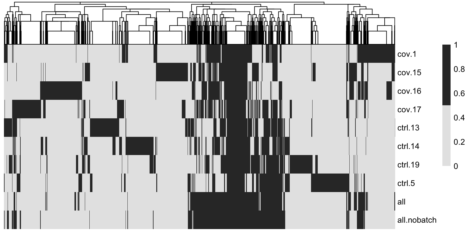
As you can see, there are a lot of genes that are variable in just one dataset. There are also some genes in the gene set that was selected using all the data without blocking samples, that are not variable in any of the individual datasets. These are most likely genes driven by batch effects.
The best way to select features for integration is to combine the information on variable genes across the dataset. This is what we have in the all section where the information on variable features in the different datasets is combined.
Discuss
Did you understand the difference between running variable gene selection per dataset and combining them vs running it on all samples together. Can you think of any situation where it would be best to run it on all samples and a situation where it should be done by batch?
For all downstream integration we will use this set of genes so that it is comparable across the methods. We already used that set of genes in the dimensionality reduction exercise to run scaling and pca.
We also store the variable gene information in the object for use furhter down the line.
metadata(sce)$hvgs = hvgs2 fastMNN
The mutual nearest neighbors (MNN) approach within the scran package utilizes a novel approach to adjust for batch effects. The fastMNN() function returns a representation of the data with reduced dimensionality, which can be used in a similar fashion to other lower-dimensional representations such as PCA. In particular, this representation can be used for downstream methods such as clustering. The BNPARAM can be used to specify the specific nearest neighbors method to use from the BiocNeighbors package. Here we make use of the Annoy library via the BiocNeighbors::AnnoyParam() argument. We save the reduced-dimension MNN representation into the reducedDims slot of our sce object.
mnn_out <- batchelor::fastMNN(sce, subset.row = hvgs, batch = factor(sce$sample), k = 20, d = 50)
Caution
fastMNN() does not produce a batch-corrected expression matrix.
We will take the reduced dimension in the new mnn_out object and add it into the original sce object.
mnn_dim <- reducedDim(mnn_out, "corrected")
reducedDim(sce, "MNN") <- mnn_dim
We can observe that a new assay slot is now created under the name MNN.
reducedDims(sce)List of length 9
names(9): PCA UMAP tSNE_on_PCA UMAP_on_PCA ... KNN UMAP_on_Graph MNNThus, the result from fastMNN() should solely be treated as a reduced dimensionality representation, suitable for direct plotting, TSNE/UMAP, clustering, and trajectory analysis that relies on such results.
set.seed(42)
sce <- runTSNE(sce, dimred = "MNN", n_dimred = 50, perplexity = 30, name = "tSNE_on_MNN")
sce <- runUMAP(sce, dimred = "MNN", n_dimred = 50, ncomponents = 2, name = "UMAP_on_MNN")
We can now plot the unintegrated and the integrated space reduced dimensions.
wrap_plots(
    plotReducedDim(sce, dimred = "PCA", colour_by = "sample", point_size = 0.6) + ggplot2::ggtitle(label = "PCA"),
    plotReducedDim(sce, dimred = "tSNE_on_PCA", colour_by = "sample", point_size = 0.6) + ggplot2::ggtitle(label = "tSNE_on_PCA"),
    plotReducedDim(sce, dimred = "UMAP_on_PCA", colour_by = "sample", point_size = 0.6) + ggplot2::ggtitle(label = "UMAP_on_PCA"),
    plotReducedDim(sce, dimred = "MNN", colour_by = "sample", point_size = 0.6) + ggplot2::ggtitle(label = "MNN"),
    plotReducedDim(sce, dimred = "tSNE_on_MNN", colour_by = "sample", point_size = 0.6) + ggplot2::ggtitle(label = "tSNE_on_MNN"),
    plotReducedDim(sce, dimred = "UMAP_on_MNN", colour_by = "sample", point_size = 0.6) + ggplot2::ggtitle(label = "UMAP_on_MNN"),
    ncol = 3
) + plot_layout(guides = "collect")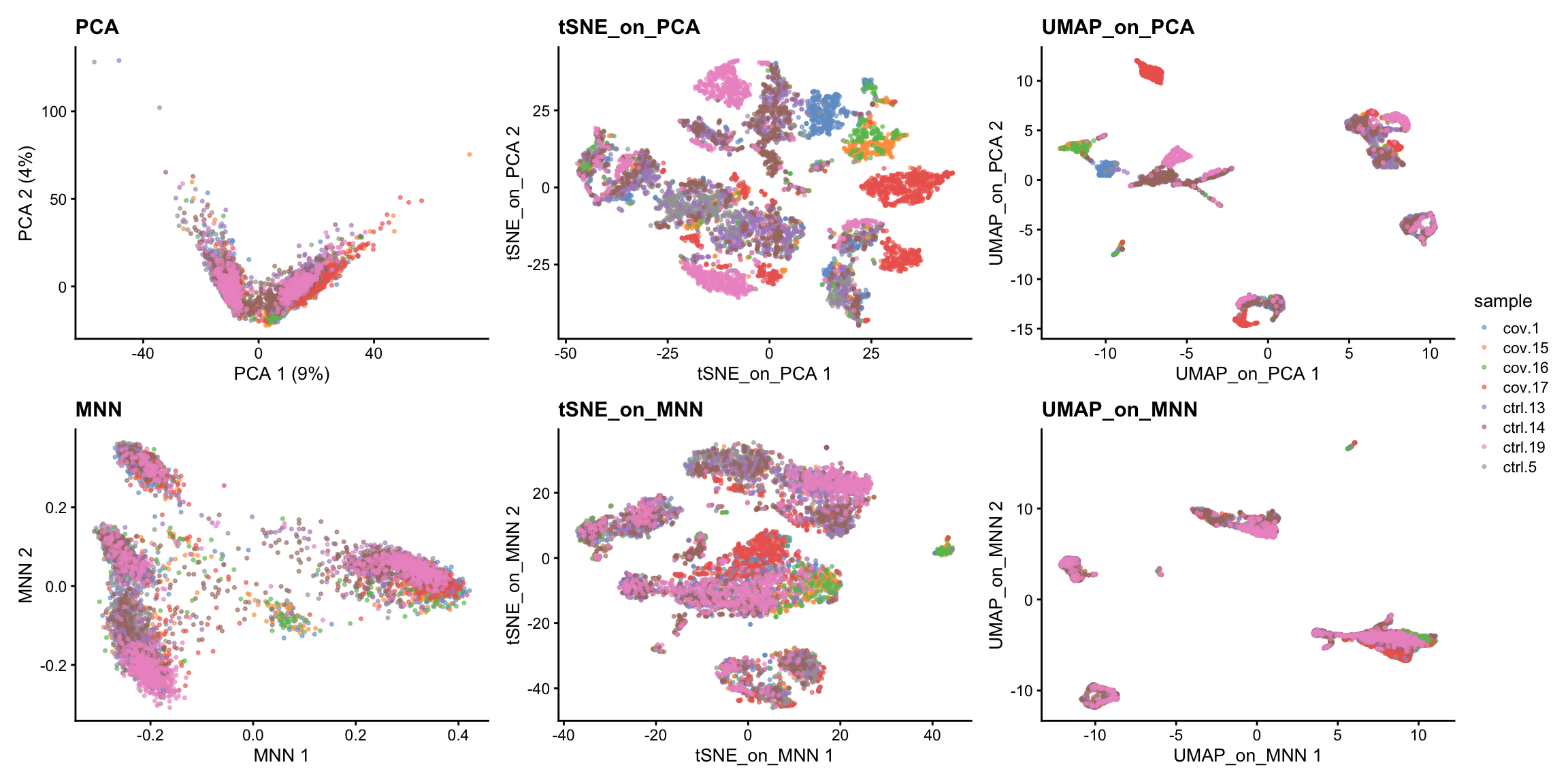
Let’s plot some marker genes for different cell types onto the embedding.
| Markers | Cell Type |
|---|---|
| CD3E | T cells |
| CD3E CD4 | CD4+ T cells |
| CD3E CD8A | CD8+ T cells |
| GNLY, NKG7 | NK cells |
| MS4A1 | B cells |
| CD14, LYZ, CST3, MS4A7 | CD14+ Monocytes |
| FCGR3A, LYZ, CST3, MS4A7 | FCGR3A+ Monocytes |
| FCER1A, CST3 | DCs |
plotlist <- list()
for (i in c("CD3E", "CD4", "CD8A", "NKG7", "GNLY", "MS4A1", "CD14", "LYZ", "MS4A7", "FCGR3A", "CST3", "FCER1A")) {
    plotlist[[i]] <- plotReducedDim(sce, dimred = "UMAP_on_MNN", colour_by = i, by_exprs_values = "logcounts", point_size = 0.6) +
        scale_fill_gradientn(colours = colorRampPalette(c("grey90", "orange3", "firebrick", "firebrick", "red", "red"))(10)) +
        ggtitle(label = i) + theme(plot.title = element_text(size = 20))
}
wrap_plots(plotlist = plotlist, ncol = 3)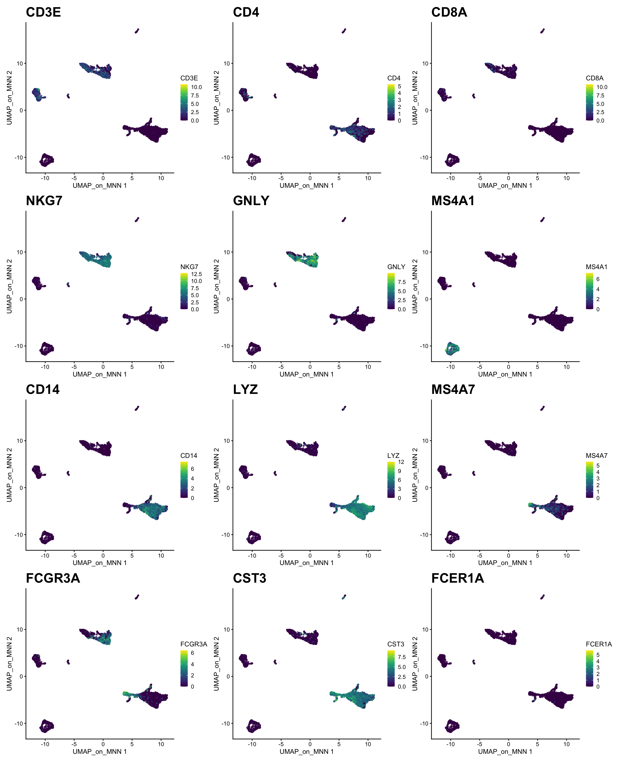
3 Harmony
An alternative method for integration is Harmony, for more details on the method, please se their paper Nat. Methods. This method runs the integration on a dimensionality reduction, in most applications the PCA. So first, we prefer to have scaling and PCA with the same set of genes that were used for the CCA integration, which we ran earlier.
library(harmony)

reducedDimNames(sce)
[1] "PCA" "UMAP" "tSNE_on_PCA"
[4] "UMAP_on_PCA" "UMAP10_on_PCA" "UMAP_on_ScaleData"
[7] "KNN" "UMAP_on_Graph" "MNN"
[10] "tSNE_on_MNN" "UMAP_on_MNN" sce <- RunHarmony(
sce,
group.by.vars = "sample",
reduction.save = "harmony",
reduction = "PCA",
dims.use = 1:50
)
# Here we use all PCs computed from Harmony for UMAP calculation
sce <- runUMAP(sce, dimred = "harmony", n_dimred = 50, ncomponents = 2, name = "UMAP_on_Harmony")
plotReducedDim(sce, dimred = "UMAP_on_Harmony", colour_by = "sample", point_size = 0.6) + ggplot2::ggtitle(label = "UMAP_on_Harmony")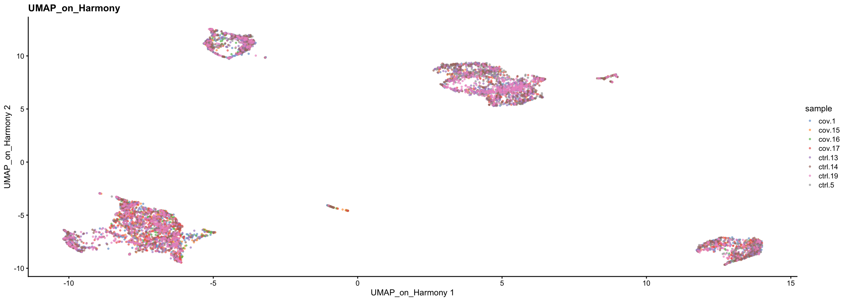
4 Scanorama
Another integration method is Scanorama (see Nat. Biotech.). This method is implemented in python, but we can run it through the Reticulate package.
We will run it with the same set of variable genes, but first we have to create a list of all the objects per sample.
scelist <- lapply(unique(sce$sample), function(x) {
    x <- t(as.matrix(assay(sce, "logcounts")[hvgs,sce$sample == x]))
})
genelist =  rep(list(hvgs),length(scelist))

lapply(scelist, dim)
[[1]]
[1] 805 2000
[[2]]
[1] 522 2000
[[3]]
[1] 348 2000
[[4]]
[1] 1018 2000
[[5]]
[1] 948 2000
[[6]]
[1] 1103 2000
[[7]]
[1] 913 2000
[[8]]
[1] 1070 2000Scanorama is implemented in python, but through reticulate we can load python packages and run python functions. In this case we also use the basilisk package for a more clean activation of python environment.
At the top of this script, we set the variable condapath to point to the conda environment where scanorama is included.
# run scanorama via basilisk with scelist and genelist as input.
integrated.data = basiliskRun(env=condapath, fun=function(datas, genes) {
  scanorama <- reticulate::import("scanorama")
  output <- scanorama$integrate(datasets_full = datas,
                                         genes_list = genes )
  return(output)
}, datas = scelist, genes = genelist, testload="scanorama")
Found 2000 genes among all datasets
[[0. 0.49616858 0.39942529 0.33988212 0.45838509 0.32670807
0.28322981 0.13364486]
[0. 0. 0.74425287 0.26245211 0.35337553 0.21072797
0.18199234 0.13793103]
[0. 0. 0. 0.23563218 0.43103448 0.42241379
0.29022989 0.26149425]
[0. 0. 0. 0. 0.18565401 0.06385069
0.10805501 0.15046729]
[0. 0. 0. 0. 0. 0.86814346
0.60337553 0.1635514 ]
[0. 0. 0. 0. 0. 0.
0.79238441 0.40841121]
[0. 0. 0. 0. 0. 0.
0. 0.68691589]
[0. 0. 0. 0. 0. 0.
0. 0. ]]
Processing datasets (4, 5)
Processing datasets (5, 6)
Processing datasets (1, 2)
Processing datasets (6, 7)
Processing datasets (4, 6)
Processing datasets (0, 1)
Processing datasets (0, 4)
Processing datasets (2, 4)
Processing datasets (2, 5)
Processing datasets (5, 7)
Processing datasets (0, 2)
Processing datasets (1, 4)
Processing datasets (0, 3)
Processing datasets (0, 5)
Processing datasets (2, 6)
Processing datasets (0, 6)
Processing datasets (1, 3)
Processing datasets (2, 7)
Processing datasets (2, 3)
Processing datasets (1, 5)
Processing datasets (3, 4)
Processing datasets (1, 6)
Processing datasets (4, 7)
Processing datasets (3, 7)
Processing datasets (1, 7)
Processing datasets (0, 7)
Processing datasets (3, 6)intdimred <- do.call(rbind, integrated.data[[1]])
colnames(intdimred) <- paste0("PC_", 1:100)
rownames(intdimred) <- colnames(logcounts(sce))
# Add standard deviations in order to draw Elbow Plots
stdevs <- apply(intdimred, MARGIN = 2, FUN = sd)
attr(intdimred, "varExplained") <- stdevs
reducedDim(sce, "Scanorama") <- intdimred
# Here we use all PCs computed from Scanorama for UMAP calculation
sce <- runUMAP(sce, dimred = "Scanorama", n_dimred = 50, ncomponents = 2, name = "UMAP_on_Scanorama")
plotReducedDim(sce, dimred = "UMAP_on_Scanorama", colour_by = "sample", point_size = 0.6) + ggplot2::ggtitle(label = "UMAP_on_Scanorama")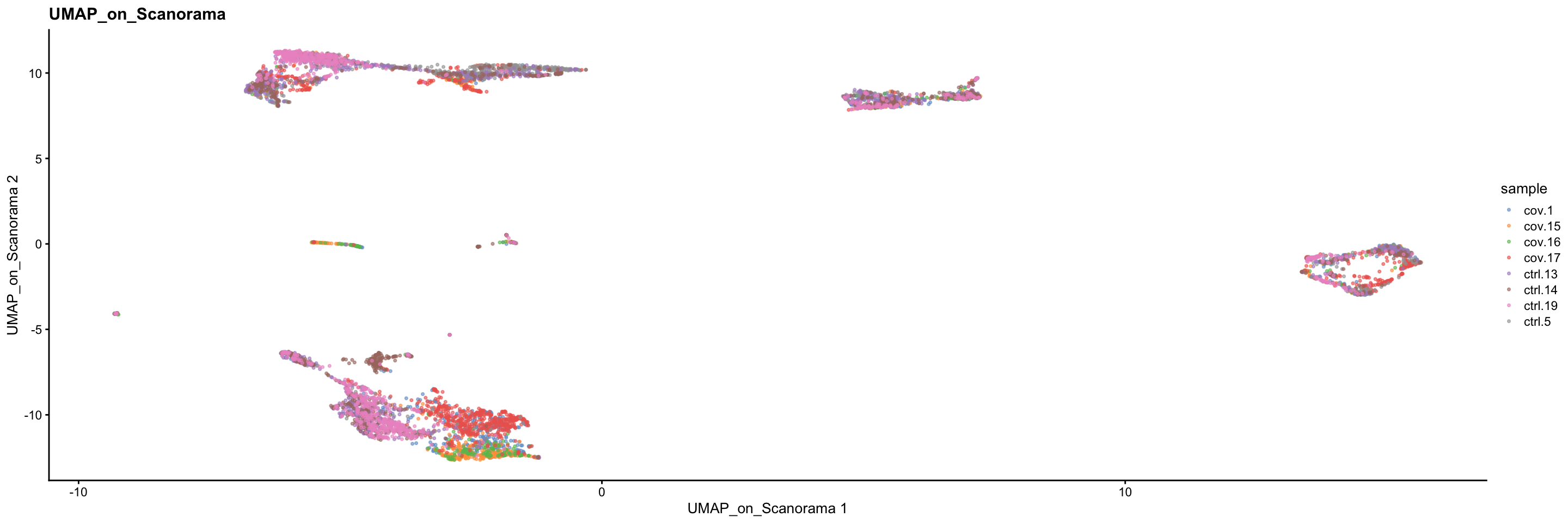
5 Overview all methods
Now we will plot UMAPS with all three integration methods side by side.
p1 <- plotReducedDim(sce, dimred = "UMAP_on_PCA", colour_by = "sample", point_size = 0.6) + ggplot2::ggtitle(label = "UMAP_on_PCA")
p2 <- plotReducedDim(sce, dimred = "UMAP_on_MNN", colour_by = "sample", point_size = 0.6) + ggplot2::ggtitle(label = "UMAP_on_MNN")
p3 <- plotReducedDim(sce, dimred = "UMAP_on_Harmony", colour_by = "sample", point_size = 0.6) + ggplot2::ggtitle(label = "UMAP_on_Harmony")
p4 <- plotReducedDim(sce, dimred = "UMAP_on_Scanorama", colour_by = "sample", point_size = 0.6) + ggplot2::ggtitle(label = "UMAP_on_Scanorama")

wrap_plots(p1, p2, p3, p4, nrow = 2) +
    plot_layout(guides = "collect")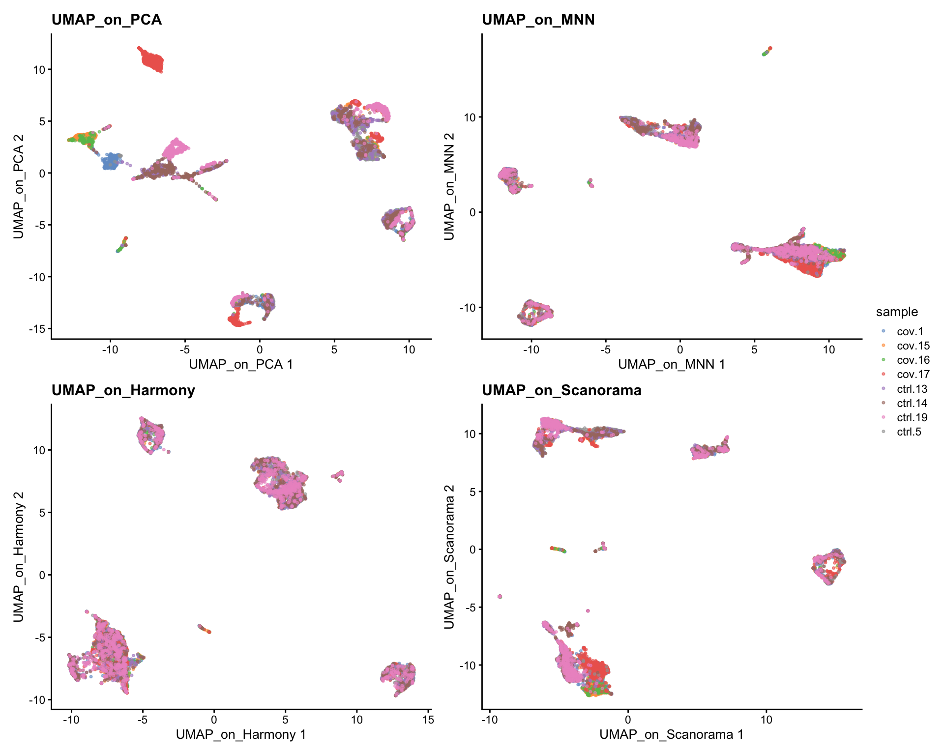
Discuss
Look at the different integration results, which one do you think looks the best? How would you motivate selecting one method over the other? How do you think you could best evaluate if the integration worked well?
Let’s save the integrated data for further analysis.
saveRDS(sce, "data/covid/results/bioc_covid_qc_dr_int.rds")6 Session info
Click here
sessionInfo()R version 4.3.3 (2024-02-29)
Platform: x86_64-conda-linux-gnu (64-bit)
Running under: Ubuntu 20.04.6 LTS
Matrix products: default
BLAS/LAPACK: /usr/local/conda/envs/seurat/lib/libopenblasp-r0.3.28.so; LAPACK version 3.12.0
locale:
[1] LC_CTYPE=en_US.UTF-8 LC_NUMERIC=C
[3] LC_TIME=en_US.UTF-8 LC_COLLATE=en_US.UTF-8
[5] LC_MONETARY=en_US.UTF-8 LC_MESSAGES=en_US.UTF-8
[7] LC_PAPER=en_US.UTF-8 LC_NAME=C
[9] LC_ADDRESS=C LC_TELEPHONE=C
[11] LC_MEASUREMENT=en_US.UTF-8 LC_IDENTIFICATION=C
time zone: Etc/UTC
tzcode source: system (glibc)
attached base packages:
[1] stats4 stats graphics grDevices utils datasets methods
[8] base
other attached packages:
[1] basilisk_1.14.1 harmony_1.2.1
[3] Rcpp_1.0.14 batchelor_1.18.0
[5] patchwork_1.3.0 scran_1.30.0
[7] scater_1.30.1 ggplot2_3.5.1
[9] scuttle_1.12.0 SingleCellExperiment_1.24.0
[11] SummarizedExperiment_1.32.0 Biobase_2.62.0
[13] GenomicRanges_1.54.1 GenomeInfoDb_1.38.1
[15] IRanges_2.36.0 S4Vectors_0.40.2
[17] BiocGenerics_0.48.1 MatrixGenerics_1.14.0
[19] matrixStats_1.5.0
loaded via a namespace (and not attached):
[1] bitops_1.0-9 gridExtra_2.3
[3] rlang_1.1.5 magrittr_2.0.3
[5] RcppAnnoy_0.0.22 compiler_4.3.3
[7] dir.expiry_1.10.0 DelayedMatrixStats_1.24.0
[9] png_0.1-8 vctrs_0.6.5
[11] pkgconfig_2.0.3 crayon_1.5.3
[13] fastmap_1.2.0 XVector_0.42.0
[15] labeling_0.4.3 rmarkdown_2.29
[17] ggbeeswarm_0.7.2 xfun_0.50
[19] bluster_1.12.0 zlibbioc_1.48.0
[21] beachmat_2.18.0 jsonlite_1.8.9
[23] DelayedArray_0.28.0 BiocParallel_1.36.0
[25] irlba_2.3.5.1 parallel_4.3.3
[27] cluster_2.1.8 R6_2.6.1
[29] RColorBrewer_1.1-3 limma_3.58.1
[31] reticulate_1.40.0 knitr_1.49
[33] Matrix_1.6-5 igraph_2.0.3
[35] tidyselect_1.2.1 abind_1.4-5
[37] yaml_2.3.10 viridis_0.6.5
[39] codetools_0.2-20 lattice_0.22-6
[41] tibble_3.2.1 basilisk.utils_1.14.1
[43] withr_3.0.2 evaluate_1.0.3
[45] Rtsne_0.17 pillar_1.10.1
[47] filelock_1.0.3 generics_0.1.3
[49] RCurl_1.98-1.16 sparseMatrixStats_1.14.0
[51] munsell_0.5.1 scales_1.3.0
[53] RhpcBLASctl_0.23-42 glue_1.8.0
[55] metapod_1.10.0 pheatmap_1.0.12
[57] tools_4.3.3 BiocNeighbors_1.20.0
[59] ScaledMatrix_1.10.0 locfit_1.5-9.11
[61] cowplot_1.1.3 grid_4.3.3
[63] edgeR_4.0.16 colorspace_2.1-1
[65] GenomeInfoDbData_1.2.11 beeswarm_0.4.0
[67] BiocSingular_1.18.0 vipor_0.4.7
[69] cli_3.6.4 rsvd_1.0.5
[71] S4Arrays_1.2.0 viridisLite_0.4.2
[73] dplyr_1.1.4 uwot_0.2.2
[75] ResidualMatrix_1.12.0 gtable_0.3.6
[77] digest_0.6.37 SparseArray_1.2.2
[79] ggrepel_0.9.6 dqrng_0.3.2
[81] htmlwidgets_1.6.4 farver_2.1.2
[83] htmltools_0.5.8.1 lifecycle_1.0.4
[85] statmod_1.5.0