class: center, middle, inverse, title-slide .title[ # Matrices, Data Frames, and Lists ] .author[ ### Guilherme Dias ] --- exclude: true count: false <link href="https://fonts.googleapis.com/css?family=Roboto|Source+Sans+Pro:300,400,600|Ubuntu+Mono&subset=latin-ext" rel="stylesheet"> <link rel="stylesheet" href="https://use.fontawesome.com/releases/v5.3.1/css/all.css" integrity="sha384-mzrmE5qonljUremFsqc01SB46JvROS7bZs3IO2EmfFsd15uHvIt+Y8vEf7N7fWAU" crossorigin="anonymous"> --- name: puzzle # Where would you store... .pull-left-50[ ### 1. A count table 20,000 genes × 6 samples. All numbers. ### 2. A sample sheet ID, strain, sex, weight, treated? Text, numbers, `TRUE`/`FALSE`. ### 3. Your whole experiment Both tables, the date, your notes, your plots. ] -- .pull-right-50[ <br> ### A vector? ❌ One type. One dimension. <br> ### We need bigger boxes 📦 ] --- name: containers # Three containers <br><br> | | Container | Like a... | |:-:|:----------|:----------| | 🧊 | **matrix** | ice-cube tray | | 📋 | **data frame** | spreadsheet | | 🎒 | **list** | backpack | --- name: matrices # 🧊 Matrices Rows × columns, **one type**. A count table: ``` r counts <- matrix(c( 120, 135, 40, 52, 300, 280, 310, 295, 15, 22, 180, 165, 2100, 1950, 2240, 2010), nrow = 4, byrow = TRUE) rownames(counts) <- c("BRCA1", "TP53", "MYC", "GAPDH") colnames(counts) <- c("WT1", "WT2", "KO1", "KO2") counts dim(counts) ``` ``` ## WT1 WT2 KO1 KO2 ## BRCA1 120 135 40 52 ## TP53 300 280 310 295 ## MYC 15 22 180 165 ## GAPDH 2100 1950 2240 2010 ## [1] 4 4 ``` --- name: matrices_indexing # Matrices: indexing `[row, column]`. Leave one empty to get everything. ``` r counts["MYC", "KO1"] # one value counts["MYC", ] # one gene, all samples counts[, c("KO1", "KO2")] ``` ``` ## [1] 180 ## WT1 WT2 KO1 KO2 ## 15 22 180 165 ## KO1 KO2 ## BRCA1 40 52 ## TP53 310 295 ## MYC 180 165 ## GAPDH 2240 2010 ``` -- Conditions work too: ``` r counts[counts[, "KO1"] > 100, ] # genes with > 100 counts in KO1 ``` ``` ## WT1 WT2 KO1 KO2 ## TP53 300 280 310 295 ## MYC 15 22 180 165 ## GAPDH 2100 1950 2240 2010 ``` --- name: matrices_calc # Matrices: calculating Operations work on every element: ``` r log2(counts + 1) ``` ``` ## WT1 WT2 KO1 KO2 ## BRCA1 6.918863 7.087463 5.357552 5.727920 ## TP53 8.233620 8.134426 8.280771 8.209453 ## MYC 4.000000 4.523562 7.499846 7.375039 ## GAPDH 11.036860 10.929998 11.129927 10.973697 ``` -- Sums and means per row or column: ``` r colSums(counts) # library size per sample rowMeans(counts) # mean per gene apply(counts, 1, max) # any function: 1 = rows, 2 = columns ``` ``` ## WT1 WT2 KO1 KO2 ## 2535 2387 2770 2522 ## BRCA1 TP53 MYC GAPDH ## 86.75 296.25 95.50 2075.00 ## BRCA1 TP53 MYC GAPDH ## 135 310 180 2240 ``` --- name: matrices_combine # Matrices: combining and flipping ``` r cbind(counts, KO3 = c(48, 305, 171, 2150)) # add a sample (column) ``` ``` ## WT1 WT2 KO1 KO2 KO3 ## BRCA1 120 135 40 52 48 ## TP53 300 280 310 295 305 ## MYC 15 22 180 165 171 ## GAPDH 2100 1950 2240 2010 2150 ``` -- ``` r t(counts) # transpose: samples become rows ``` ``` ## BRCA1 TP53 MYC GAPDH ## WT1 120 300 15 2100 ## WT2 135 280 22 1950 ## KO1 40 310 180 2240 ## KO2 52 295 165 2010 ``` --- name: data_frames_1 # 📋 Data frames - A **table**: like a spreadsheet. - Each column is a vector, with **its own type**. - All columns have the **same length**. <center> .size-70[ 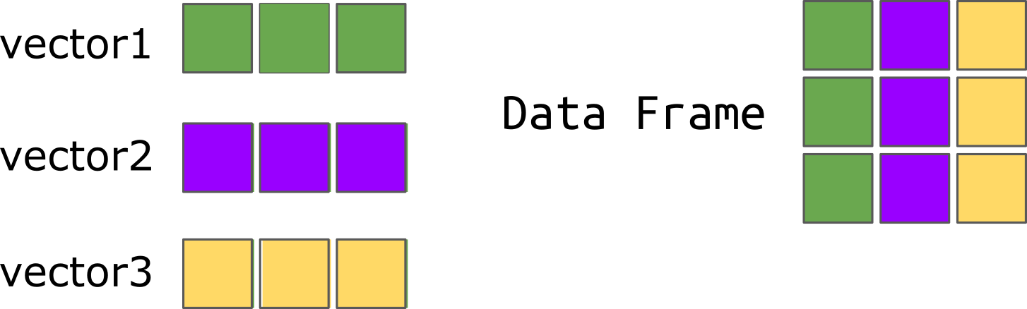 ] </center> --- name: data_frames_create # Data frames: creating A sample sheet. **Name your columns!** ``` r samples <- data.frame( sample = c("WT1", "WT2", "KO1", "KO2"), strain = c("WT", "WT", "KO", "KO"), sex = c("F", "M", "F", "M"), weight = c(22.1, 25.4, 21.8, 26.3), treated = c(FALSE, TRUE, FALSE, TRUE) ) samples ``` ``` ## sample strain sex weight treated ## 1 WT1 WT F 22.1 FALSE ## 2 WT2 WT M 25.4 TRUE ## 3 KO1 KO F 21.8 FALSE ## 4 KO2 KO M 26.3 TRUE ``` --- name: data_frames_inspect # Data frames: a first look ``` r str(samples) # structure: columns and types ``` ``` ## 'data.frame': 4 obs. of 5 variables: ## $ sample : chr "WT1" "WT2" "KO1" "KO2" ## $ strain : chr "WT" "WT" "KO" "KO" ## $ sex : chr "F" "M" "F" "M" ## $ weight : num 22.1 25.4 21.8 26.3 ## $ treated: logi FALSE TRUE FALSE TRUE ``` -- ``` r summary(samples) ``` ``` ## sample strain sex weight ## Length:4 Length:4 Length:4 Min. :21.80 ## Class :character Class :character Class :character 1st Qu.:22.02 ## Mode :character Mode :character Mode :character Median :23.75 ## Mean :23.90 ## 3rd Qu.:25.62 ## Max. :26.30 ## treated ## Mode :logical ## FALSE:2 ## TRUE :2 ## ## ## ``` .footnote[Also useful: `head()`, `nrow()`, `ncol()`, `dim()`, `colnames()`.] --- name: data_frames_accessing # Data frames: accessing `$` gets a column (a vector): ``` r samples$weight mean(samples$weight) ``` ``` ## [1] 22.1 25.4 21.8 26.3 ## [1] 23.9 ``` -- `[row, column]` works like a matrix: ``` r samples[2, ] # second row samples[, c("sample", "weight")] # two columns samples[3, "weight"] # one value ``` ``` ## sample strain sex weight treated ## 2 WT2 WT M 25.4 TRUE ## sample weight ## 1 WT1 22.1 ## 2 WT2 25.4 ## 3 KO1 21.8 ## 4 KO2 26.3 ## [1] 21.8 ``` --- name: data_frames_filter # Data frames: filtering rows A condition picks the rows: ``` r samples[samples$strain == "KO", ] samples[samples$strain == "KO" & samples$weight > 25, ] samples$sample[samples$treated] # just the names ``` ``` ## sample strain sex weight treated ## 3 KO1 KO F 21.8 FALSE ## 4 KO2 KO M 26.3 TRUE ## sample strain sex weight treated ## 4 KO2 KO M 26.3 TRUE ## [1] "WT2" "KO2" ``` This is your Excel filter. In one line, and it's saved in your script. --- name: data_frames_add # Data frames: adding columns ``` r samples$heavy <- samples$weight > 24 # a new logical column samples$strain <- factor(samples$strain, levels = c("WT", "KO")) samples ``` ``` ## sample strain sex weight treated heavy ## 1 WT1 WT F 22.1 FALSE FALSE ## 2 WT2 WT M 25.4 TRUE TRUE ## 3 KO1 KO F 21.8 FALSE FALSE ## 4 KO2 KO M 26.3 TRUE TRUE ``` -- Calculations on columns work on all rows at once, just like vectors. --- name: data_frames_merging # Data frames: merging Another table, **in a different order**: ``` r batches <- data.frame(sample = c("KO1", "WT1", "KO2", "WT2"), batch = c(1, 1, 2, 2)) ``` -- `merge()` matches rows by a **key** column, not by position: ``` r merge(samples[, c("sample", "strain")], batches, by = "sample") ``` ``` ## sample strain batch ## 1 KO1 KO 1 ## 2 KO2 KO 2 ## 3 WT1 WT 1 ## 4 WT2 WT 2 ``` .content-box-yellow[ Never paste tables side by side and hope the rows line up. Merge by ID. ] --- name: data_frames_missing # Data frames: missing values ``` r samples$weight[2] <- NA # a lost measurement colSums(is.na(samples)) # NAs per column na.omit(samples) # drop rows with any NA ``` ``` ## sample strain sex weight treated heavy ## 0 0 0 1 0 0 ## sample strain sex weight treated heavy ## 1 WT1 WT F 22.1 FALSE FALSE ## 3 KO1 KO F 21.8 FALSE FALSE ## 4 KO2 KO M 26.3 TRUE TRUE ``` --- name: lists_1 # 🎒 Lists A list holds **anything**: vectors, tables, other lists. ``` r experiment <- list( name = "MYC knockout pilot", date = "2026-03-14", samples = samples, counts = counts ) str(experiment, max.level = 1) ``` ``` ## List of 4 ## $ name : chr "MYC knockout pilot" ## $ date : chr "2026-03-14" ## $ samples:'data.frame': 4 obs. of 6 variables: ## $ counts : num [1:4, 1:4] 120 300 15 2100 135 280 22 1950 40 310 ... ## ..- attr(*, "dimnames")=List of 2 ``` --- name: lists_subsetting # Lists: `[[ ]]` vs `[ ]` .pull-left-50[ ``` r experiment[["name"]] class(experiment[["name"]]) ``` ``` ## [1] "MYC knockout pilot" ## [1] "character" ``` `[[ ]]` takes the thing **out**. ] .pull-right-50[ ``` r experiment["name"] class(experiment["name"]) ``` ``` ## $name ## [1] "MYC knockout pilot" ## ## [1] "list" ``` `[ ]` gives a **smaller list**. ] <div style="clear: both;"></div> <img src="images/salt_list.png" width="60%" style="display: block; margin: auto auto auto 0;" /> --- name: lists_dollar # Lists: `$` and digging deeper `$` works like `[[ ]]` for named elements: ``` r experiment$name experiment$samples$sample # a column inside a data frame inside a list experiment$counts["MYC", ] ``` ``` ## [1] "MYC knockout pilot" ## [1] "WT1" "WT2" "KO1" "KO2" ## WT1 WT2 KO1 KO2 ## 15 22 180 165 ``` -- Add or remove elements: ``` r experiment$notes <- "KO2 was sluggish on day 3" experiment$date <- NULL # remove names(experiment) ``` ``` ## [1] "name" "samples" "counts" "notes" ``` --- name: lists_results # Lists are everywhere Many functions return a list. A t-test, for example: ``` r wt <- c(22.1, 25.4, 23.0, 24.2) ko <- c(21.8, 26.3, 27.1, 26.0) res <- t.test(ko, wt) is.list(res) names(res) res$p.value ``` ``` ## [1] TRUE ## [1] "statistic" "parameter" "p.value" "conf.int" "estimate" ## [6] "null.value" "stderr" "alternative" "method" "data.name" ## [1] 0.2956134 ``` Knowing lists = knowing how to get your results out. --- name: recap # Recap | | Shape | Types | Get things out | |:--|:------|:------|:---------------| | 🧊 **matrix** | rows × columns | one | `m["MYC", ]`, `m[, 2]` | | 📋 **data frame** | rows × columns | one per column | `df$weight`, `df[df$x > 1, ]` | | 🎒 **list** | anything | anything | `l$samples`, `l[["name"]]` | <br> **Remember:** - Filter rows with conditions, not by hand. - Merge tables by ID, not by position. - `[[ ]]` takes out, `[ ]` keeps a list. <!-- --------------------- Do not edit this and below --------------------- --> --- name: end_slide class: end-slide, middle count: false # See you at the next lecture! .end-text[ <p class="smaller"> <span class="small" style="line-height: 1.2;">Graphics from </span><img src="./assets/freepik.jpg" style="max-height:20px; vertical-align:middle;"><br> Created: 12-Nov-2026 • <a href="https://www.scilifelab.se/">SciLifeLab</a> • <a href="https://nbis.se/">NBIS</a> </p> ]