Basic statistic
R Programming Foundation for Data Analysis
1 Introduction
In this lab, we will use statistics to gain a deeper understanding and insight into the dataset. Through statistical methods, we can evaluate data quality, identify patterns, and detect any outliers that may be present. You will apply several descriptive measures to explore and summarize the dataset, allowing for a more informed analysis.
2 Generating the Data
We create a dataset which consists of:
- Two numerical variables (Normally distributed).
- Three categorical.
n samples with [0-100]% missing data). You can also adjust these values to create a new dataset. We will talk about functions tomorrow.
# Function to generate the data
generate_dataset <- function(n, na_frac) {

  # Set seed for reproducibility
  set.seed(123)

  # Gender variable
  Gender <- sample(c('Male', 'Female'), n, replace = TRUE)

  # Continuous Variable 1 with shifted distribution between genders
  Variable_1 <- ifelse(Gender == 'Male', rnorm(n, mean = 55, sd = 10), rnorm(n, mean = 45, sd = 10))

  # Continuous Variable 2: negative correlation with Variable_1 for one of the sexes
  Variable_2 <- ifelse(Gender == 'Male', -0.5 * Variable_1 + rnorm(n, mean = 10, sd = 5),
                       0.5 * Variable_1 + rnorm(n, mean = 10, sd = 5))

  # Introduce NA values (10% of the data by default)
  Variable_1[sample(1:n, round(n*na_frac))] <- NA
  Variable_2[sample(1:n, round(n*na_frac))] <- NA

  # Introduce outliers
  Variable_1[c(n)] <- max(Variable_1, na.rm = T) + sd(Variable_1, na.rm = T)
  Variable_1[c(round(n)/2)] <- min(Variable_1, na.rm = T) - sd(Variable_1, na.rm = T)

  Variable_2[c(n)] <- max(Variable_2, na.rm = T) + sd(Variable_2, na.rm = T)
  Variable_2[c(round(n)/2)] <- min(Variable_2, na.rm = T) - sd(Variable_2, na.rm = T)

  # Categorical variables with more levels for Spearman correlation
  Category_1 <- sample(c('Category_A', 'Category_B', 'Category_C', 'Category_D', 'Category_E'), n, replace = TRUE)
  Category_2 <- sample(c('Group1', 'Group2', 'Group3'), n, replace = TRUE)

  # Create data frame
  dataset <- data.frame(Variable_1, Variable_2, Category_1, Category_2, Gender)
  return(dataset)
}

n <- 1000 # Number of samples (observation).
na_frac <- 0.1 # Introducing missing values in the dataset.
dataset <- generate_dataset(n, na_frac = na_frac )- Check the content of the dataset.
- How many rows and columns do you have?
head(dataset)
dim(dataset)
## Variable_1 Variable_2 Category_1 Category_2 Gender
## 1 48.98107 -17.884574 Category_E Group3 Male
## 2 45.06301 -9.659943 Category_E Group1 Male
## 3 NA -26.156498 Category_C Group2 Male
## 4 51.27069 34.248513 Category_C Group2 Female
## 5 39.90833 -6.082244 Category_B Group1 Male
## 6 66.27214 42.492134 Category_B Group3 Female
## [1] 1000 53 Measures of Central Tendency
3.1 Mean
mean_var1 <- mean(dataset$Variable_1)
mean_var2 <- mean(dataset$Variable_2)
mean_var1
mean_var2
## [1] NA
## [1] NAWhat is the
meanvalue ofVariable_1andVariable_2?Is it NA? Why?
How many NA values do you find in your dataset?
n_na <- sum(is.na(dataset))
sprintf('There are %g missing values', n_na)
## [1] "There are 199 missing values"- Can you fix it?
Click to expand
To handle theNAvalues, you can setna.rm = TRUEin the functionmean(x, na.rm = T), which removes the queries withNAvalues.
hist(). You will learn more about plots in Basic Graphics lecture.
hist(dataset$Variable_1, main = 'Distribution of Variable_1', xlab = 'Variable_1')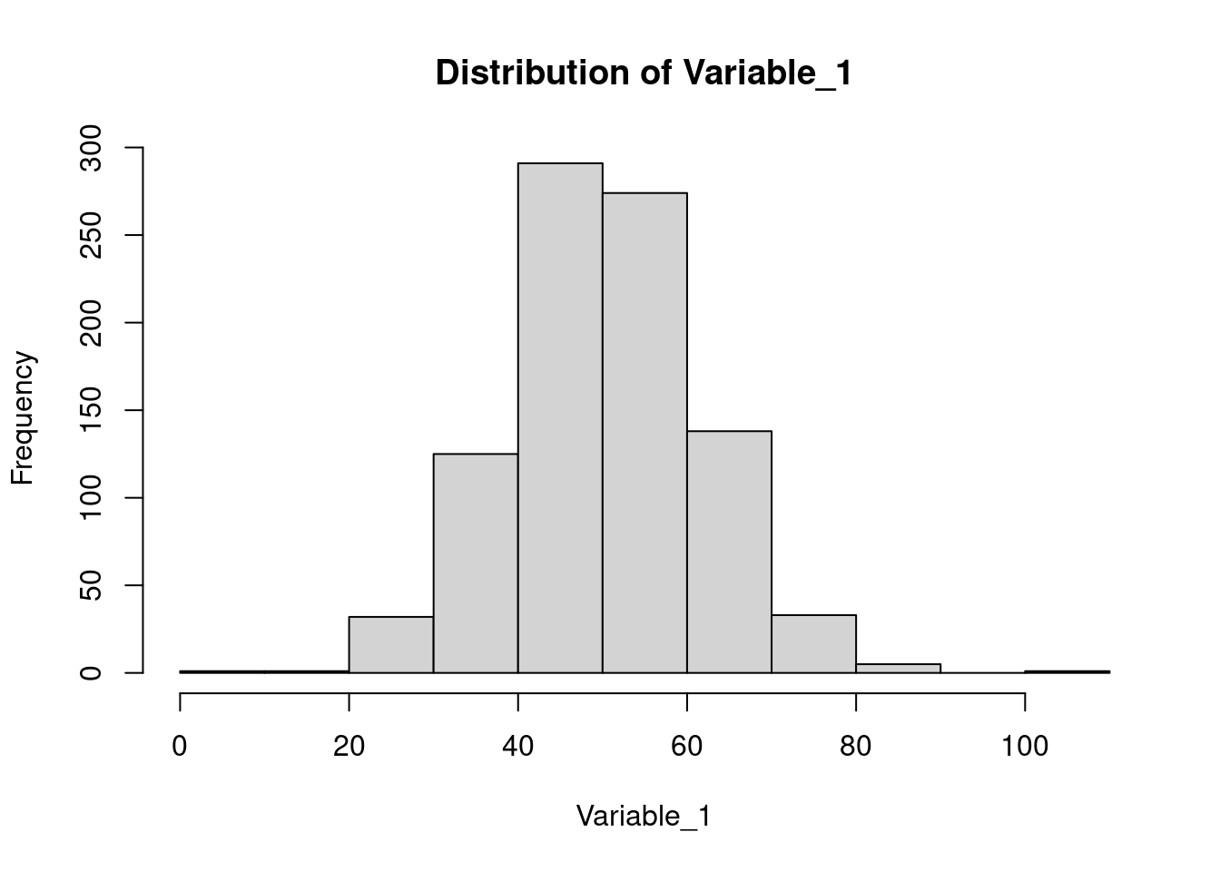
dataset_f <- dataset[(dataset$Gender == 'Female'), ]
dataset_m <- dataset[(dataset$Gender == 'Male'), ]
hist(dataset_f$Variable_1, main = 'Female', xlab = 'Variable_1')
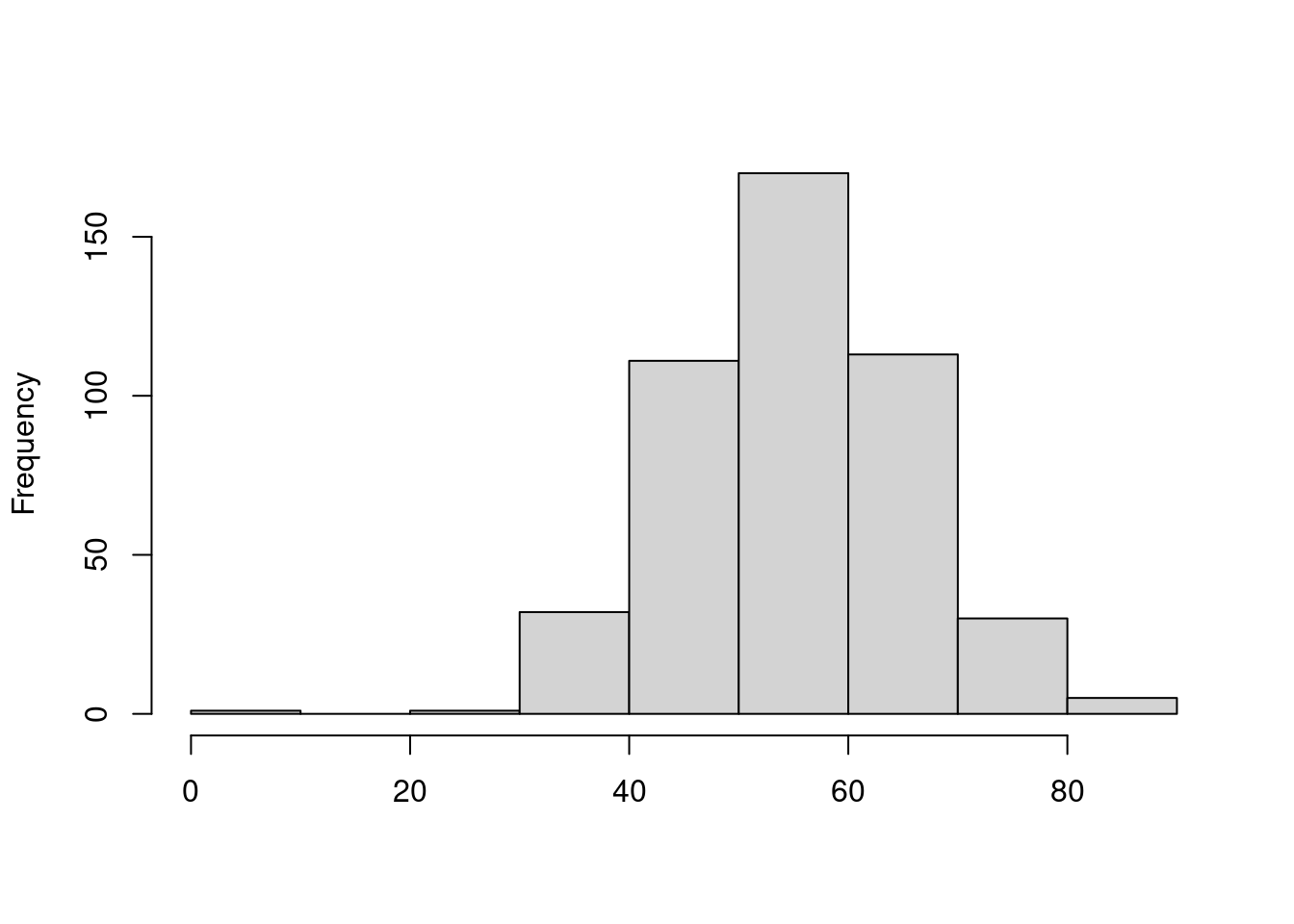
hist(dataset_m$Variable_1, main = '', xlab = '')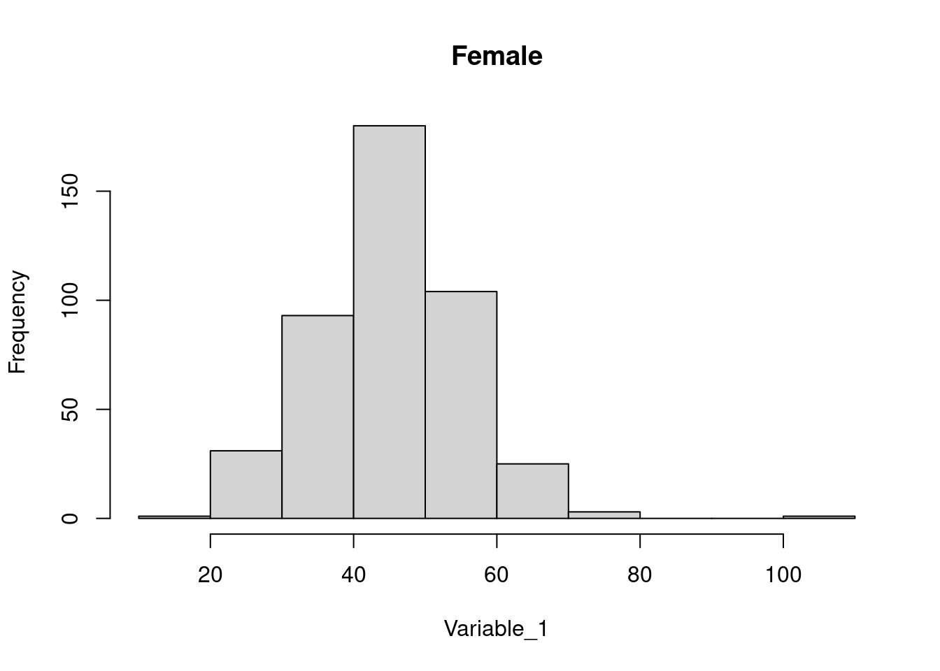
3.2 Median
median_var1 <- median(dataset$Variable_1, na.rm = T)
median_var2 <- median(dataset$Variable_2, na.rm = T)
median_var1
median_var2
## [1] 50.004
## [1] -4.7408054 Measures of Spread
4.1 Range
We can find the range of values in numerical variables.
range_var1 <- range(dataset$Variable_1, na.rm = TRUE)
range_var2 <- range(dataset$Variable_2, na.rm = TRUE)
range_var1
range_var2
## [1] 3.119354 100.190691
## [1] -65.86148 83.70804
table(dataset$Category_1)
table(dataset[,c('Category_1', 'Category_2')])
table(dataset[,c('Category_1', 'Category_2', 'Gender')])
##
## Category_A Category_B Category_C Category_D Category_E
## 203 201 204 194 198
## Category_2
## Category_1 Group1 Group2 Group3
## Category_A 80 65 58
## Category_B 72 62 67
## Category_C 73 71 60
## Category_D 62 63 69
## Category_E 64 68 66
## , , Gender = Female
##
## Category_2
## Category_1 Group1 Group2 Group3
## Category_A 41 34 27
## Category_B 35 31 30
## Category_C 33 43 28
## Category_D 32 32 43
## Category_E 23 38 24
##
## , , Gender = Male
##
## Category_2
## Category_1 Group1 Group2 Group3
## Category_A 39 31 31
## Category_B 37 31 37
## Category_C 40 28 32
## Category_D 30 31 26
## Category_E 41 30 424.2 Interquartile.
Calculate the following for Variable_1:
- Min.
- Median.
- Max.
- Quantiles (q1:25% and q2:75%) by using
quantilefunction.
- Interquartile range (q3 - q1).
na.rm = T)
min_val <- min(dataset$Variable_1, na.rm = T)
q1 <- quantile(dataset$Variable_1, 0.25, na.rm = T)
median_val <- median(dataset$Variable_1, na.rm = T)
q3 <- quantile(dataset$Variable_1, 0.75, na.rm = T)
max_val <- max(dataset$Variable_1, na.rm = T)
print('Variable_1 range:')
c(min_val, q1, median_val, q3, max_val)

# Interqurtile:
print('Interquartile:')
iqr_val1 <- q3 - q1
unname(iqr_val1)
# or
iqr_val1 <- IQR(dataset$Variable_1, na.rm = T)
iqr_val1
## [1] "Variable_1 range:"
## 25% 75%
## 3.119354 42.793157 50.003998 57.990869 100.190691
## [1] "Interquartile:"
## [1] 15.19771
## [1] 15.197714.3 Standard deviation
sdis a built-in function in R to calculate standard deviation.- Calculate standard deviation of
Variable_1for males and females separately.
na.rm = T)
sd_var1_f <- sd(dataset_f$Variable_1, na.rm = TRUE)
sd_var1_m <- sd(dataset_m$Variable_1, na.rm = TRUE)
sd_var1_f
sd_var1_m
## [1] 10.21548
## [1] 10.566164.4 Variance
varis a built-in function in R to calculate variance.
- Calculate variance of
Variable_1for males and females separately.
na.rm = T).
var_var1_f <- var(dataset_f$Variable_1, na.rm = TRUE)
var_var1_m <- var(dataset_m$Variable_1, na.rm = TRUE)
var_var1_f
var_var1_m
## [1] 104.356
## [1] 111.64375 Correlation
5.1 Pearson’s correlation
- Let’s check the correlation of
Variable_1andVariable_2by Pearson’s method implemented incorfunction. You can specify the method bymethod = 'pearson'.
Note: Here we handle the missing values a bit differently. In cor function, you control the missing values (NA) by setting use = 'complete.obs' which means to include observations that there are values for both variables. In other words, rows with NA in either of the values will be excluded.
pearson_correlation <- cor(dataset$Variable_1, dataset$Variable_2, use = 'complete.obs', method = "pearson")
pearson_correlation
## [1] -0.4171403- You can also plot the values in a simple plot using
plotfunction. How do you interpret the results?
plot(dataset$Variable_1, dataset$Variable_2, main = 'Variable_1 vs Variable_2', xlab = 'Variable_1', ylab = 'Variable_2')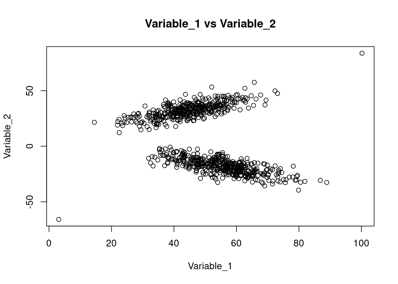
5.2 Spearman’s correlation
- You can calculate Spearman’s correlation using the same function (
cor) for both numerical and categorical data.
- Check the result of Spearman’s correlation and Pearson’s correlation for
Variable_1andVariable_2.
- Calculate the correlation between
Category_1andVariable_1. ConsiderCategory_1with ordinal variable such as level of satisfaction labeled as Category_A to E.
cor. You first need to encode the values as factors (the values are presented in form of levels) by as.factor. Then by converting the vector (e.g. dataset$Category_1) to numeric by as.numeric function, you can pass it to cor function.
# Spearman correlation for numerical variables
spearman_corr_numeric <- cor(dataset$Variable_1, dataset$Variable_2, use = "complete.obs", method = "spearman")

# Spearman correlation between numeric and categorical variables
spearman_corr_cat_var1 <- cor(as.numeric(as.factor(dataset$Category_1)), dataset$Variable_1, use = "complete.obs", method = "spearman")
spearman_corr_cat_var2 <- cor(as.numeric(as.factor(dataset$Category_1)), dataset$Variable_2, use = "complete.obs", method = "spearman")

spearman_corr_numeric
spearman_corr_cat_var1
spearman_corr_cat_var2
## [1] -0.4284315
## [1] 0.02013907
## [1] 0.0280211- Plot categorical data using
plotfunction can be fun! If you pass the categorical as factor (as.factor(dataset$Category_1)) together with a numerical values, you will generate a boxplot.
plot((as.factor(dataset$Category_1)), dataset$Variable_1)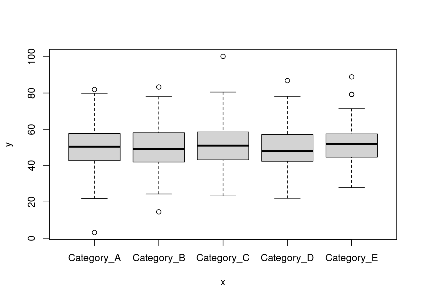
5.3 Optional exercise
- Calculate the correlation between
GenderandVariable_1,Genderas well asVariable_2.
cor_gender_var1 <- cor(as.numeric(as.factor(dataset$Gender)), dataset$Variable_1, use = 'complete.obs', method = 'spearman')
cor_gender_var2 <- cor(as.numeric(as.factor(dataset$Gender)), dataset$Variable_2, use = 'complete.obs', method = 'spearman')
cor_gender_var1
cor_gender_var2
## [1] 0.4465193
## [1] -0.8657672- Now plot
GendervsVariable_1orVariable_2. How do you interpret the result?
plot((as.factor(dataset$Gender)), dataset$Variable_1)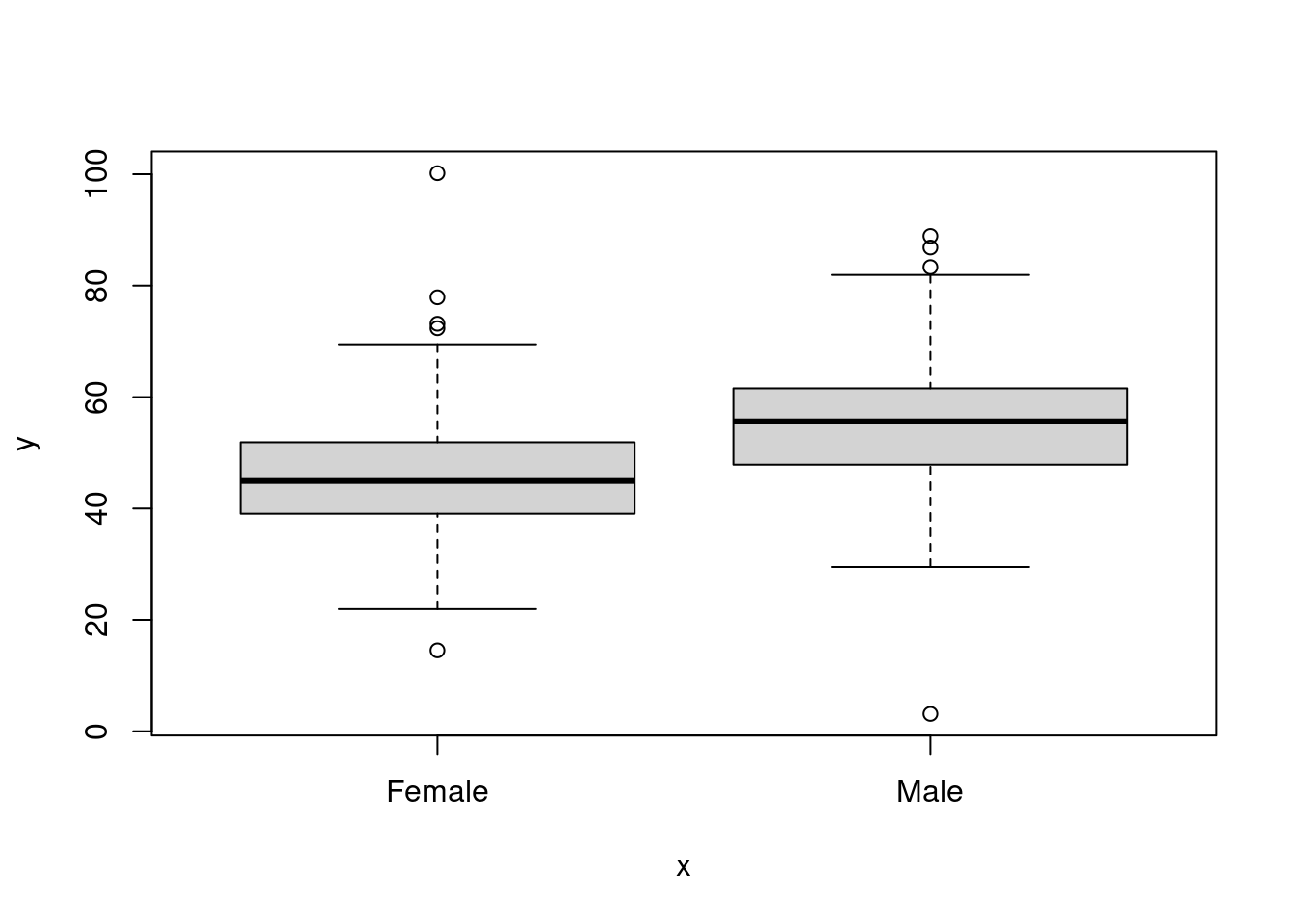
plot(as.factor(dataset$Gender), dataset$Variable_2)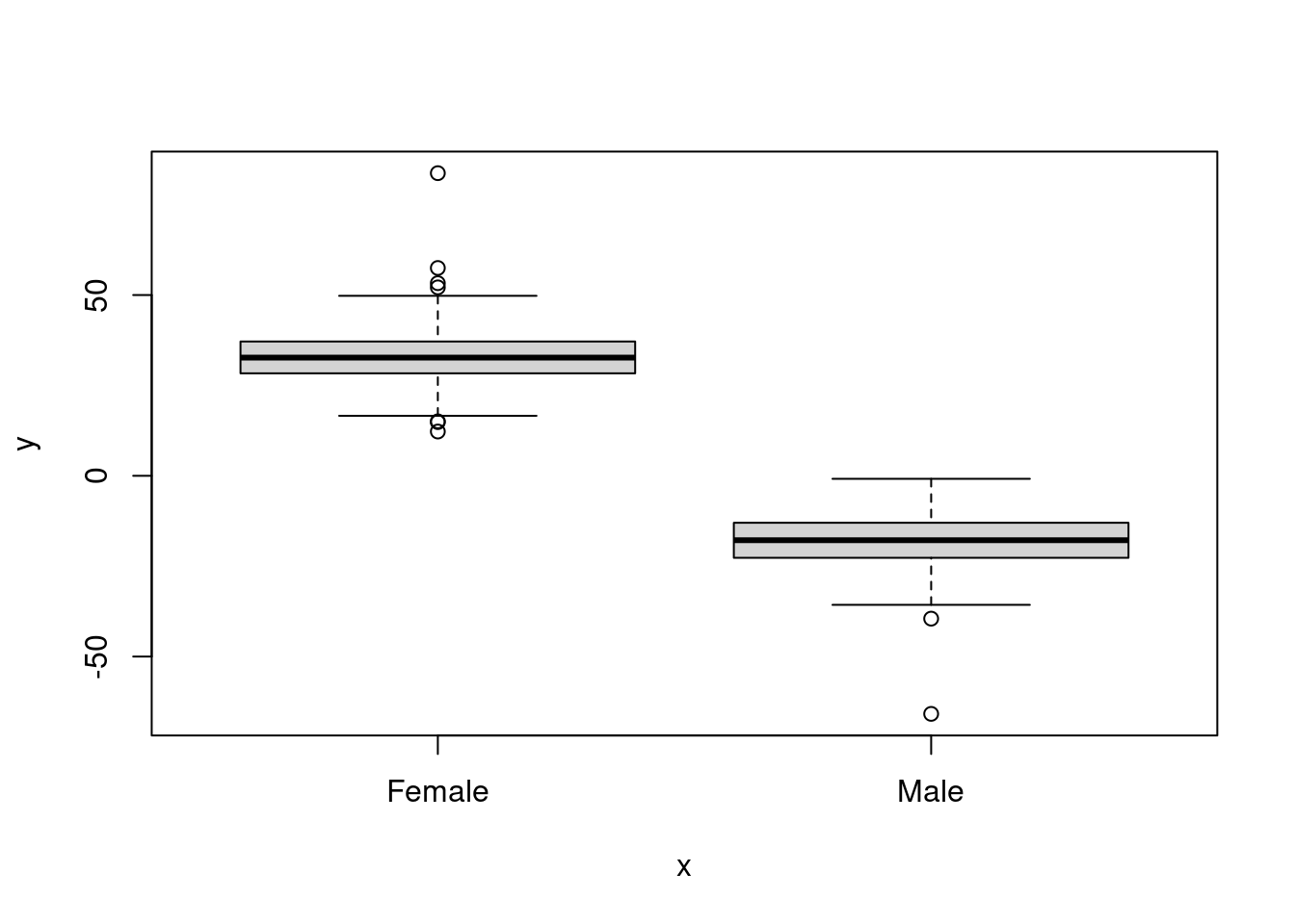
6 Bonus
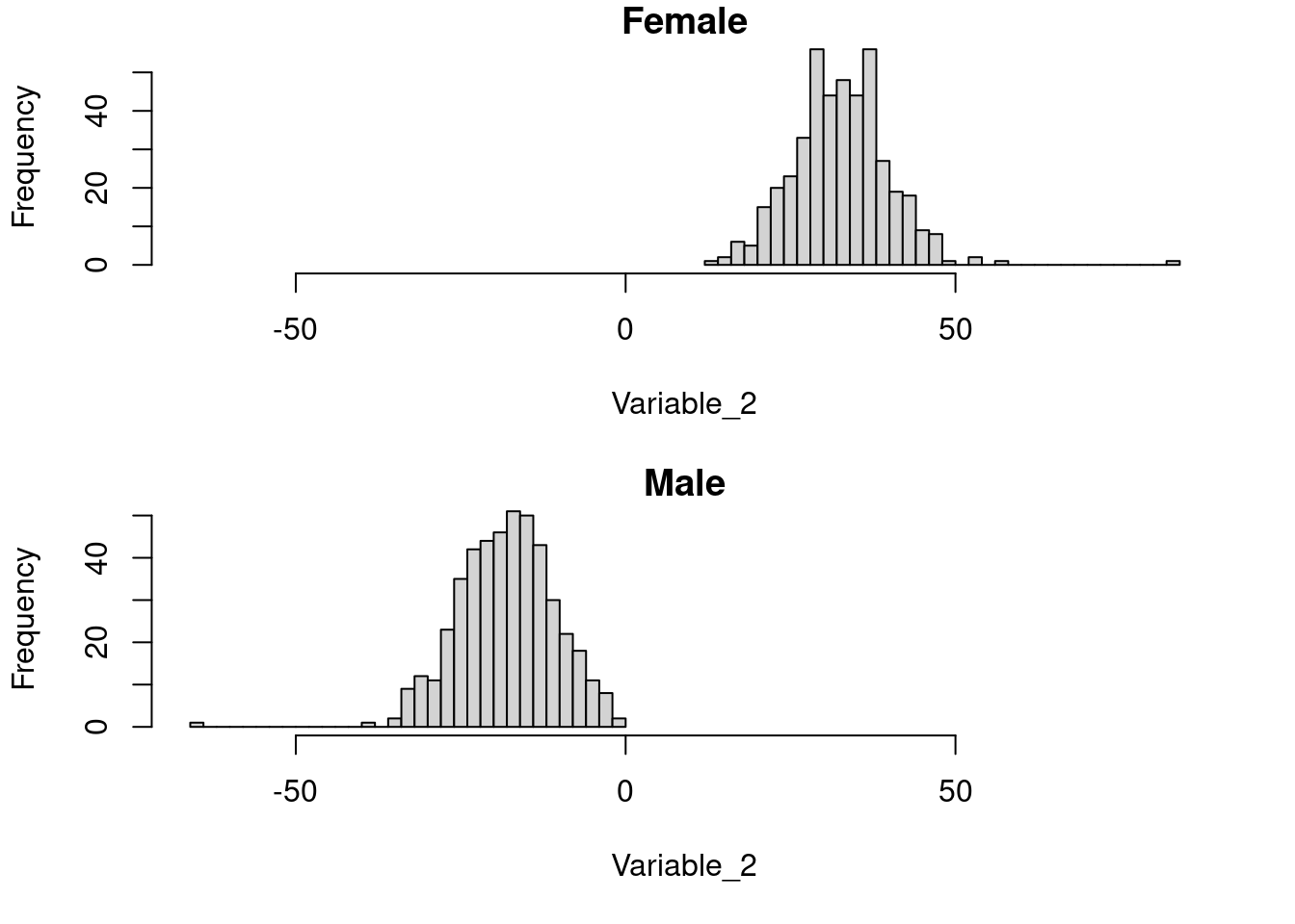
You can show both histograms (males and females) in the same plot. You will learn about this in “Basic Graphics”.
par(mfrow = c(2,1), mar = c(5, 4, 1, 2) + 0.1)
range_val <- c(min(dataset$Variable_2, na.rm = T), max(dataset$Variable_2, na.rm = T) )
hist(dataset_f$Variable_2, main = 'Female', xlab = 'Variable_2', xlim = range_val, breaks = 30)
hist(dataset_m$Variable_2, main = 'Male', xlab = 'Variable_2', xlim = range_val, breaks = 30)