RShiny Lab: Part III
Workshop on Plotting in R
Lokesh Mano • 18-Jan-2022
In this section of the lab, we will try to go into making an app step-by-step. The idea basically is to first have a plan/backbone of the page that we want and then to go on populating the page in a step-wise manner!
1 Aesthetics
There is one part of the shiny app that could also be argued as the important part of an Rshiny app is its aesthetics. We will not cover any of this in the course unfortunately as there will be no time, if we go into it. But there are many tutorials and exercises to learn this part. I will list some of the sources where you can learn how to make your app look pretty and nice.
Here is a link from the webinar series of Rstudio explaining the different aspects of the aesthetics in the shiny app that you can work on!
This is a similar tutorial how to write a calendar app given at NBIS RaukR course
Shiny themes that you can use after you set everything
2 Covid App
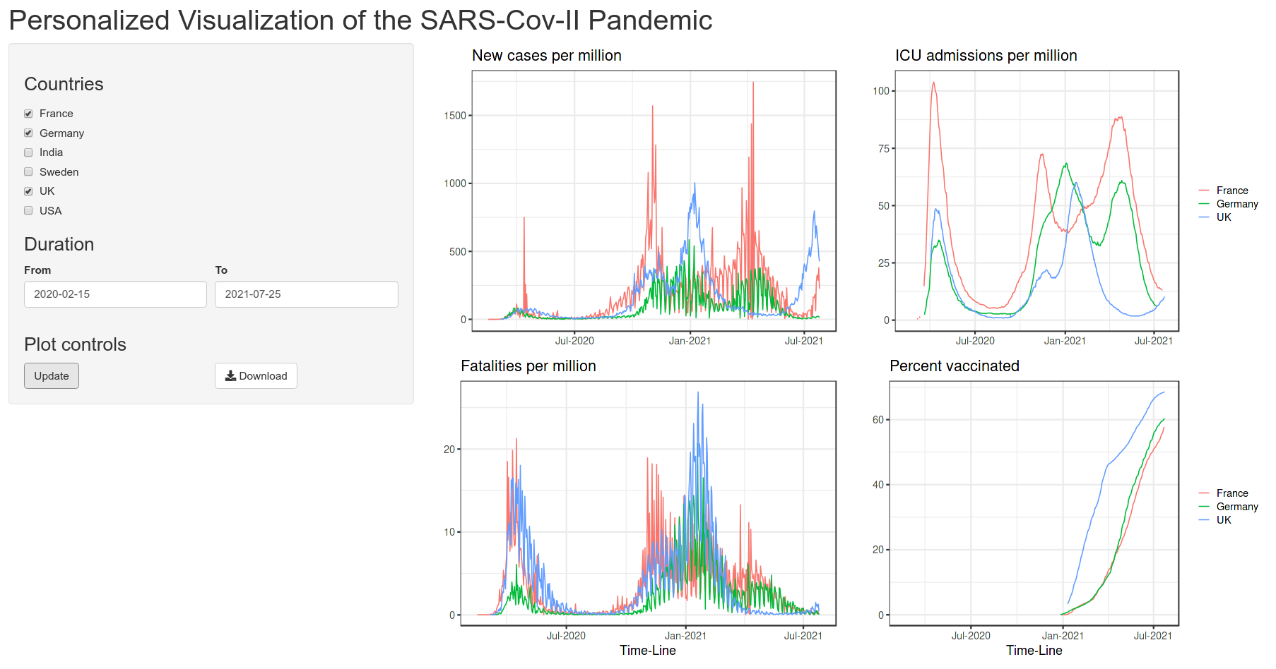
In the following steps, we will try to make an app that is basically on the data available on the current pandemic and the vaccinations from Our world in Data. Here, we basically want to choose the data available from 6 different countries that are: France, Germany, India, Sweden, UK and USA. We would also like to give the option to choose which date range that one would like to visualize between 2020-02-15 to 2021-07-25.
Topics covered
- UI layout using pre-defined function (pageWithSidebar)
- Input and output widgets and reactivity
- Use of date-time
- Customized ggplot
- Download image files
- Update inputs using observe
- Validating inputs with custom error messages
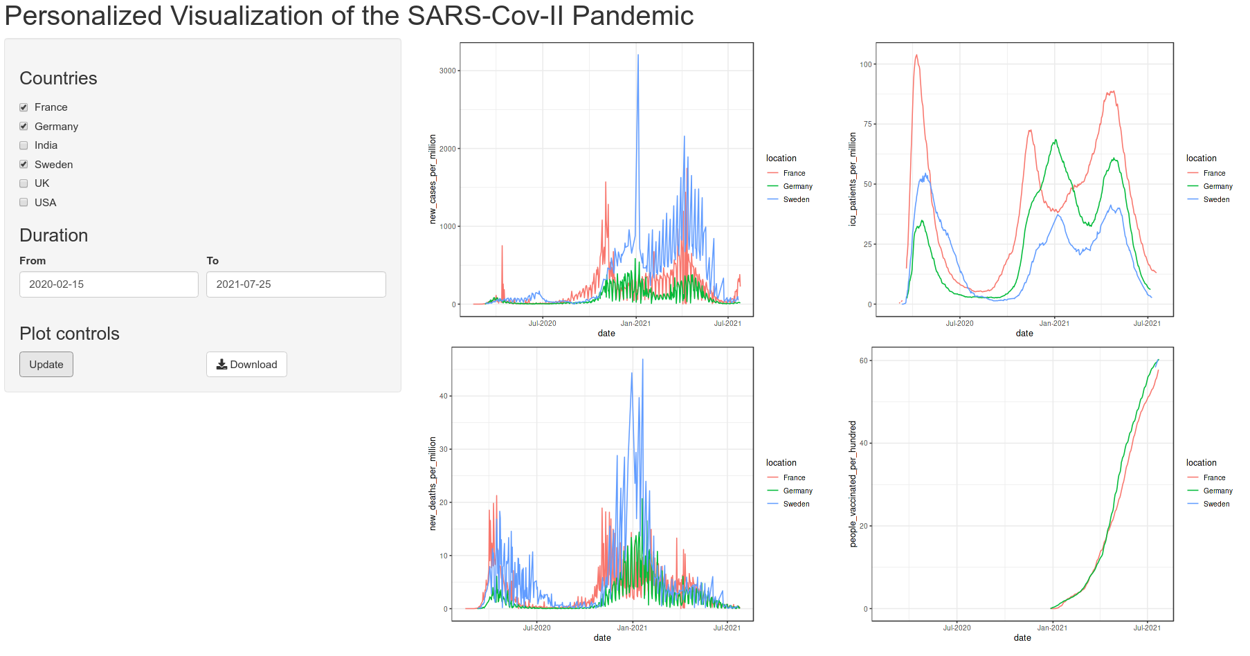
Below is the quick view of the app that we are aiming to achieve:
3 Data structure
First let us take a quick look at the data and how it is formatted. For this exercise we will use the file shiny_app_data.csv.
cov_data <- read.table("data/shiny_app_data.csv", sep = ",", header = T)
head(cov_data)
output
##   location       date new_cases_per_million new_deaths_per_million
## 1   France 2020-02-15                 0.015                  0.015
## 2   France 2020-02-26                 0.059                  0.015
## 3   France 2020-03-02                 0.903                  0.015
## 4   France 2020-03-03                 0.311                  0.015
## 5   France 2020-03-05                 2.043                  0.044
## 6   France 2020-03-06                 2.812                  0.030
##   icu_patients_per_million people_vaccinated_per_hundred
## 1                       NA                            NA
## 2                       NA                            NA
## 3                       NA                            NA
## 4                       NA                            NA
## 5                    0.340                            NA
## 6                    0.577                            NA
It is a simple comma-separated file with 6 columns: location, date, new_cases_per_million, new_deaths_per_million, icu_patients_per_million and people_vaccinated_per_hundred. Now, the idea is that we will use the first two columns as input values where user can choose the countries and the date range for which they would like to see how the pandemic was and then we make the four plots accordingly! For making these animated plots in the app, we would need the following packages: shiny, cowplot, tidyverse, ggplot and shinythemes.
4 Example plot
Now let us take a quick look at how to make one of these plots! The following code should produce a similar plot as below:
library(gganimate)
library(ggplot2)

cov_data <- read.table("data/shiny_app_data.csv", sep = ",", header = T)
cov_data$date <- as.Date(cov_data$date)

cov_data %>%
  ggplot(aes(x= date, y=new_cases_per_million, group = location, color = location)) +
  geom_line() +
  geom_point() +
  theme_bw() +
  scale_x_date(date_labels = "%b-%Y") +
  transition_reveal(date)
Here the transition_reveal() from gganimate makes the plot into an animation based on the date x axis data. But this usually takes some time in the background to calculate! For the sake of time, I will skip the animation part in building this app. This is just to show you that these kinds of functions can come very much handy when you make these interactive plots in Rshiny!
5 Building the app
Now, let us go ahead and start building the app! First, let us get the data and the libraries into the app in the right form as we would want it.
library(shiny)
library(tidyverse)
library(ggplot2)
library(dplyr)
library(cowplot)

cov_data <- read.table("data/shiny_app_data.csv", sep = ",", header = T)
cov_data$date <- as.Date(cov_data$date)
5.1 Layout
We need to first have a plan for the app page, which UI elements to include and how they will be laid out and structured. My plan is as shown in the preview image.
There is a horizontal top bar for the title and two columns below. The left column will contain the input widgets and control. The right column will contain the plot output. Since, this is a commonly used layout, it is available as a predefined function in shiny called pageWithSidebar(). It takes three arguments headerPanel, sidebarPanel and mainPanel which is self explanatory.
library(shiny)
library(tidyverse)
library(ggplot2)
library(dplyr)
library(cowplot)

cov_data <- read.table("data/shiny_app_data.csv", sep = ",", header = T)
cov_data$date <- as.Date(cov_data$date)


shinyApp(
ui=fluidPage(
  pageWithSidebar(
    headerPanel(),
    sidebarPanel(),
    mainPanel())
  ),
server=function(input,output){}
)
5.2 UI
Then we fill in the panels with widgets and contents. The way I planned this app is to have two input values from user which are the countries to visualize and the duration, as I mentioned earlier. In addition I would also like to have the Update button to control the reactivity of the plots as we have learnt in the earlier session. So, the plots should update only when the Update button is pressed. I would also like to give the user the option to download these animated plots as gif image.
Let us start with including the countries as a checkboxGroupInput() input widget. It is self-explanatory that the countries you choose in this group can be accessed in the server() to subset the data just for these countries. The function comes with its own header label, followed by choices and you can use selected to have the default choice.
shinyApp(
    ui=fluidPage(
        pageWithSidebar(
            headerPanel(title="Personalized Visualization of the SARS-Cov-II Pandemic",windowTitle="Covid Data"),
            sidebarPanel(
                checkboxGroupInput("countries", label = h3("Countries"),
                                   choices = list("France" = "France", "Germany" = "Germany", "India" = "India", "Sweden" = "Sweden", "UK" = "UK", "USA" = "USA"),
                                   selected = "USA"),
            ),
            mainPanel())
    ),
    server=function(input,output){}
)
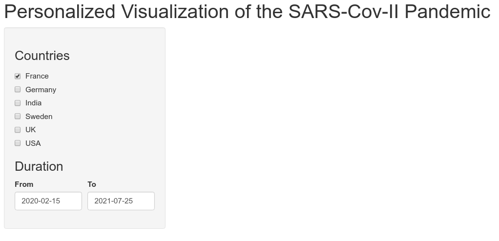
Now that we got the countries-input sorted out, let us now add the duration of the period, a user would like to visualize the data for. We can add this by doing the following:
shinyApp(
    ui=fluidPage(
        pageWithSidebar(
            headerPanel(title="Personalized Visualization of the SARS-Cov-II Pandemic",windowTitle="Covid Data"),
            sidebarPanel(
                checkboxGroupInput("countries", label = h3("Countries"),
                                   choices = list("France" = "France", "Germany" = "Germany", "India" = "India", "Sweden" = "Sweden", "UK" = "UK", "USA" = "USA"),
                                   selected = "USA"),
                h3("Duration"),
                fluidRow(
                    column(6,style=list("padding-right: 5px;"),
                           dateInput("in_duration_date_start","From",value="2020-02-15")
                    ),
                    column(6,style=list("padding-left: 5px;"),
                           dateInput("in_duration_date_end","To",value="2021-07-25")
                    )
                )
            ),
            mainPanel())
    ),
    server=function(input,output){}
)
We have defined a part of the side bar panel with a title Duration. fluidRow() is an html tag used to create rows. Above, in the side bar panel, a row is defined and two columns are defined inside. Each column is filled with date input widgets for start and end dates. We use the columns here to place date input widgets side by side. To place widgets one below the other, the columns can simply be removed.
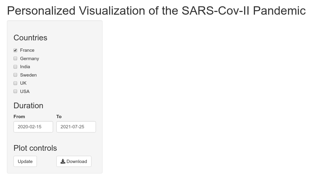
Now let us add the last part of the sidebar panel where we add actionButtons for us to be able to do Update and Download.
shinyApp(
    ui=fluidPage(
        pageWithSidebar(
            headerPanel(title="Personalized Visualization of the SARS-Cov-II Pandemic",windowTitle="Covid Data"),
            sidebarPanel(
                checkboxGroupInput("countries", label = h3("Countries"),
                                   choices = list("France" = "France", "Germany" = "Germany", "India" = "India", "Sweden" = "Sweden", "UK" = "UK", "USA" = "USA"),
                                   selected = "USA"),
                h3("Duration"),
                fluidRow(
                    column(6,style=list("padding-right: 5px;"),
                           dateInput("in_duration_date_start","From",value="2020-02-15")
                    ),
                    column(6,style=list("padding-left: 5px;"),
                           dateInput("in_duration_date_end","To",value="2021-07-25")
                    )
                ),
                h3("Plot controls"),
                fluidRow(
                    column(6,style=list("padding-right: 5px;"),
                           actionButton("click", "Update")
                    ),
                    column(6,style=list("padding-left: 5px;"),
                           downloadButton('download', 'Download')
                    ),
                )
            ),
            mainPanel()
            )
    ),
    server=function(input,output){}
)
Now we can finalize the UI part by adding the interface for the plotOutput()s. So basically we want two rows with two columns. We can add this by using fluidRow() as we have done before:
shinyApp(
    ui=fluidPage(
        pageWithSidebar(
            headerPanel(title="Personalized Visualization of the SARS-Cov-II Pandemic",windowTitle="Covid Data"),
            sidebarPanel(
                checkboxGroupInput("countries", label = h3("Countries"),
                                   choices = list("France" = "France", "Germany" = "Germany", "India" = "India", "Sweden" = "Sweden", "UK" = "UK", "USA" = "USA"),
                                   selected = "USA"),
                h3("Duration"),
                fluidRow(
                    column(6,style=list("padding-right: 5px;"),
                           dateInput("in_duration_date_start","From",value="2020-02-15")
                    ),
                    column(6,style=list("padding-left: 5px;"),
                           dateInput("in_duration_date_end","To",value="2021-07-25")
                    )
                ),
                h3("Plot controls"),
                fluidRow(
                    column(6,style=list("padding-right: 5px;"),
                           actionButton("click", "Update")
                    ),
                    column(6,style=list("padding-left: 5px;"),
                           downloadButton('download', 'Download')
                    ),
                )
            ),
            mainPanel(
                fluidRow(
                    column(width = 6, plotOutput("casesPlot",  width="100%")),
                    column(width = 6, plotOutput("hospitalPlot",  width="100%"))
                ),
                fluidRow(
                    column(width = 6, plotOutput("fatalPlot",  width="100%")),
                    column(width = 6, plotOutput("vaccinePlot",  width="100%"))
                )
            )
            )
    ),
    server=function(input,output){}
)
The UI is set for now! Now let us move-on to the server part and then eventually figure-out if we have to come back to the UI part again for changes!
5.3 Server
The first thing that I would like to do here is to make sure that the inputs we get from the user are valid for our data!
5.3.1 Error validation
As I have mentioned before, we have two inputs from the user and let us start with the country! We need to make sure that the user has selected at-least one country! For this, I would also make some changes in the ui part where I would like to show an error message, when the user has not selected a country! For this I would use conditionalPanel() where the panel appears if the condition is satisfied. Similarly, we want the selected duration to be between 2020-02-15 and 2021-07-25, so I would create another conditionalPanel() for this input. So, the ui part of the app would look like below:
 ui=fluidPage(
        pageWithSidebar(
            headerPanel(title="Personalized Visualization of the SARS-Cov-II Pandemic",windowTitle="Covid Data"),
            sidebarPanel(
                checkboxGroupInput("countries", label = h3("Countries"),
                                   choices = list("France" = "France", "Germany" = "Germany", "India" = "India", "Sweden" = "Sweden", "UK" = "UK", "USA" = "USA"),
                                   selected = "USA"),
                conditionalPanel(condition = "input.countries == ''",
                                 textOutput('error_country')),
                h3("Duration"),
                fluidRow(
                    column(6,style=list("padding-right: 5px;"),
                           dateInput("in_duration_date_start","From",value="2020-02-15")
                    ),
                    column(6,style=list("padding-left: 5px;"),
                           dateInput("in_duration_date_end","To",value="2021-07-25")
                    )
                ),
                conditionalPanel(condition = "input.in_duration_date_start < as.Date('2020-02-15') || input.in_duration_date_end < as.Date('2020-02-15') || input.in_duration_date_start > as.Date('2021-07-25') || input.in_duration_date_end > as.Date('2021-07-25')",
                                 textOutput('error_duration')),
                h3("Plot controls"),
                fluidRow(
                    column(6,style=list("padding-right: 5px;"),
                           actionButton("click", "Update")
                    ),
                    column(6,style=list("padding-left: 5px;"),
                           downloadButton('download', 'Download')
                    ),
                )
            ),
            mainPanel(
                fluidRow(
                    column(width = 6, plotOutput("casesPlot",  width="100%")),
                    column(width = 6, plotOutput("hospitalPlot",  width="100%"))
                ),
                fluidRow(
                    column(width = 6, plotOutput("fatalPlot",  width="100%")),
                    column(width = 6, plotOutput("vaccinePlot",  width="100%"))
                )
            )
          )
)
Note the syntax with input.countries inside the conditionalPanel(). This is different from how you would normally use it as input$countries within the server.
We will render the output error message in the server part when those above mentioned conditions satisfy. This I would do it in combination with the observeEvent() function in relation to our Update button in the sidebar! So, as soon as that button is clicked, we need to check if the input values are good! The actual error validation part here I do it with the combination of functions validate() and need(). So, the server would like:
server=function(input,output){

        observeEvent(input$click, {
            output$error_country <- renderText({
                shiny::validate(
                    shiny::need(input$countries != '', 'You must select at-least one country'
                    )
                )
            })
            output$error_duration <- renderText({
                shiny::validate(
                    shiny::need(input$in_duration_date_start > as.Date('2020-02-14') & input$in_duration_date_end > as.Date('2020-02-14') & input$in_duration_date_start < as.Date('2021-07-26') & input$in_duration_date_end < as.Date('2021-07-26'),
                                'You must select the duration between 2020-02-15 and 2021-07-25'
                    )
                )
            })
            shiny::req(input$countries)
        })
}
Note that the conditional statement with need() is a little different from the conditionalPanel(). The conditions we use in these two functions are basically the negation of each other. In need(): the options as we want and in conditionalPanel(): the options are suppose to check for the wrong values.
I include req() as well for the countries, so that the plots are not made when there are no countries specified.
5.3.2 Subset and plots
We subset the data of our interest simply using the filter() function from dplyr package.
server=function(input,output){

        observeEvent(input$click, {
            output$error_country <- renderText({
                shiny::validate(
                    shiny::need(input$countries != '', 'You must select at-least one country'
                    )
                )
            })
            output$error_duration <- renderText({
                shiny::validate(
                    shiny::need(input$in_duration_date_start > as.Date('2020-02-14') & input$in_duration_date_end > as.Date('2020-02-14') & input$in_duration_date_start < as.Date('2021-07-26') & input$in_duration_date_end < as.Date('2021-07-26'),
                                'You must select the duration between 2020-02-15 and 2021-07-25'
                    )
                )
            })
            shiny::req(input$countries)

            subset_covdata <- cov_data %>%
                filter(location %in% input$countries) %>%
                filter(date >= input$in_duration_date_start) %>%
                filter(date <= input$in_duration_date_end)

        })
    }
Then we use our plotting strategy that we already looked at before! We simply use that code for the four different plots that we want to populate in the mainPanel(). As you would expect, we will use the renderPlot() function to render these plots on the panel. So, finally we should have a properly working app based on the code below:
library(shiny)
library(tidyverse)
library(ggplot2)
library(dplyr)
library(cowplot)

cov_data <- read.table("data/shiny_app_data.csv", sep = ",", header = T)
cov_data$date <- as.Date(cov_data$date)

valfn_country <- function(x) if(is.null(x) | is.na(x) | x=="") return("You must select at-least one country")
valfn_date <- function(x) if(x < as.Date('2020-02-15') | x > as.Date('2021-07-25')) return("You must select the 'from' and 'to' dates between 2020-02-15 and 2021-07-25")

shinyApp(
    ui=fluidPage(
        pageWithSidebar(
            headerPanel(title="Personalized Visualization of the SARS-Cov-II Pandemic",windowTitle="Covid Data"),
            sidebarPanel(
                checkboxGroupInput("countries", label = h3("Countries"),
                                   choices = list("France" = "France", "Germany" = "Germany", "India" = "India", "Sweden" = "Sweden", "UK" = "UK", "USA" = "USA"),
                                   selected = "France"),
                conditionalPanel(condition = "input.countries == ''",
                                 textOutput('error_country')),
                h3("Duration"),
                fluidRow(
                    column(6,style=list("padding-right: 5px;"),
                           dateInput("in_duration_date_start","From",value="2020-02-15")
                    ),
                    column(6,style=list("padding-left: 5px;"),
                           dateInput("in_duration_date_end","To",value="2021-07-25")
                    )
                ),
                conditionalPanel(condition = "input.in_duration_date_start < as.Date('2020-02-15') || input.in_duration_date_end < as.Date('2020-02-15') || input.in_duration_date_start > as.Date('2021-07-25') || input.in_duration_date_end > as.Date('2021-07-25')",
                                 textOutput('error_duration')),
                h3("Plot controls"),
                fluidRow(
                    column(6,style=list("padding-right: 5px;"),
                           actionButton("click", "Update")
                    ),
                    column(6,style=list("padding-left: 5px;"),
                           downloadButton('download', 'Download')
                    ),
                )
            ),
            mainPanel(
                fluidRow(
                    column(width = 6, plotOutput("casesPlot",  width="100%")),
                    column(width = 6, plotOutput("hospitalPlot",  width="100%"))
                ),
                fluidRow(
                    column(width = 6, plotOutput("fatalPlot",  width="100%")),
                    column(width = 6, plotOutput("vaccinePlot",  width="100%"))
                )
            )
            )
    ),
    server=function(input,output){

        observeEvent(input$click, {
            output$error_country <- renderText({
                shiny::validate(
                    shiny::need(input$countries != '', 'You must select at-least one country'
                    )
                )
            })
            output$error_duration <- renderText({
                shiny::validate(
                    shiny::need(input$in_duration_date_start > as.Date('2020-02-14') & input$in_duration_date_end > as.Date('2020-02-14') & input$in_duration_date_start < as.Date('2021-07-26') & input$in_duration_date_end < as.Date('2021-07-26'),
                                'You must select the duration between 2020-02-15 and 2021-07-25'
                    )
                )
            })
            shiny::req(input$countries)

            subset_covdata <- cov_data %>%
                filter(location %in% input$countries) %>%
                filter(date >= input$in_duration_date_start) %>%
                filter(date <= input$in_duration_date_end)

            p1 <- subset_covdata %>%
                ggplot(aes(x= date, y=new_cases_per_million, group = location, color = location)) +
                geom_line() +
                theme_bw() +
                scale_x_date(date_labels = "%b-%Y")

            output$casesPlot <- renderPlot({p1})

            p2 <- subset_covdata %>%
                ggplot(aes(x= date, y=icu_patients_per_million, group = location, color = location)) +
                geom_line() +
                theme_bw() +
                scale_x_date(date_labels = "%b-%Y")

            output$hospitalPlot <- renderPlot({p2})

            p3 <- subset_covdata %>%
                ggplot(aes(x= date, y=new_deaths_per_million, group = location, color = location)) +
                geom_line() +
                theme_bw() +
                scale_x_date(date_labels = "%b-%Y")

            output$fatalPlot <- renderPlot({p3})

            p4 <- subset_covdata %>%
                ggplot(aes(x= date, y=people_vaccinated_per_hundred, group = location, color = location)) +
                geom_line() +
                theme_bw() +
                scale_x_date(date_labels = "%b-%Y")

            output$vaccinePlot <- renderPlot({p4})


        })


    }
)
Now let us make these plots look a little bit more prettier!
p1 <- subset_covdata %>%
                ggplot(aes(x= date, y=new_cases_per_million, group = location, color = location)) +
                geom_line(show.legend = F) +
                theme_bw(base_size = 16) +
                scale_x_date(date_labels = "%b-%Y") +
                xlab(label = "Time-Line") +
                theme(axis.title.y = element_blank(), axis.title.x = element_blank(), legend.title = element_blank()) +
                ggtitle(label = "New cases per million")


            output$casesPlot <- renderPlot({p1})

            p2 <- subset_covdata %>%
                ggplot(aes(x= date, y=icu_patients_per_million, group = location, color = location)) +
                geom_line() +
                theme_bw(base_size = 16) +
                scale_x_date(date_labels = "%b-%Y") +
                xlab(label = "Time-Line") +
                theme(axis.title.y = element_blank(), axis.title.x = element_blank(), legend.title = element_blank()) +
                ggtitle(label = "ICU admissions per million")

            output$hospitalPlot <- renderPlot({p2})

            p3 <- subset_covdata %>%
                ggplot(aes(x= date, y=new_deaths_per_million, group = location, color = location)) +
                geom_line(show.legend = F) +
                theme_bw(base_size = 16) +
                scale_x_date(date_labels = "%b-%Y") +
                xlab(label = "Time-Line") +
                theme(axis.title.y = element_blank(), legend.title = element_blank()) +
                ggtitle(label = "Fatalities per million")

            output$fatalPlot <- renderPlot({p3})

            p4 <- subset_covdata %>%
                ggplot(aes(x= date, y=people_vaccinated_per_hundred, group = location, color = location)) +
                geom_line() +
                theme_bw(base_size = 16) +
                scale_x_date(date_labels = "%b-%Y") +
                xlab(label = "Time-Line") +
                theme(axis.title.y = element_blank(), legend.title = element_blank()) +
                ggtitle(label = "Percent vaccinated")

            output$vaccinePlot <- renderPlot({p4})
5.3.3 Downloading
Now let us look into the last part of the app, which is to download these plots together in a PDF document. For this we use the function downloadHandler().
server=function(input,output){

        observeEvent(input$click, {
            output$error_country <- renderText({
                shiny::validate(
                    shiny::need(input$countries != '', 'You must select at-least one country'
                    )
                )
            })
            output$error_duration <- renderText({
                shiny::validate(
                    shiny::need(input$in_duration_date_start > as.Date('2020-02-14') & input$in_duration_date_end > as.Date('2020-02-14') & input$in_duration_date_start < as.Date('2021-07-26') & input$in_duration_date_end < as.Date('2021-07-26'),
                                'You must select the duration between 2020-02-15 and 2021-07-25'
                    )
                )
            })
            shiny::req(input$countries)

            subset_covdata <- cov_data %>%
                filter(location %in% input$countries) %>%
                filter(date >= input$in_duration_date_start) %>%
                filter(date <= input$in_duration_date_end)

            p1 <- subset_covdata %>%
                ggplot(aes(x= date, y=new_cases_per_million, group = location, color = location)) +
                geom_line(show.legend = F) +
                theme_bw(base_size = 16) +
                scale_x_date(date_labels = "%b-%Y") +
                xlab(label = "Time-Line") +
                theme(axis.title.y = element_blank(), axis.title.x = element_blank(), legend.title = element_blank()) +
                ggtitle(label = "New cases per million")


            output$casesPlot <- renderPlot({p1})

            p2 <- subset_covdata %>%
                ggplot(aes(x= date, y=icu_patients_per_million, group = location, color = location)) +
                geom_line() +
                theme_bw(base_size = 16) +
                scale_x_date(date_labels = "%b-%Y") +
                xlab(label = "Time-Line") +
                theme(axis.title.y = element_blank(), axis.title.x = element_blank(), legend.title = element_blank()) +
                ggtitle(label = "ICU admissions per million")

            output$hospitalPlot <- renderPlot({p2})

            p3 <- subset_covdata %>%
                ggplot(aes(x= date, y=new_deaths_per_million, group = location, color = location)) +
                geom_line(show.legend = F) +
                theme_bw(base_size = 16) +
                scale_x_date(date_labels = "%b-%Y") +
                xlab(label = "Time-Line") +
                theme(axis.title.y = element_blank(), legend.title = element_blank()) +
                ggtitle(label = "Fatalities per million")

            output$fatalPlot <- renderPlot({p3})

            p4 <- subset_covdata %>%
                ggplot(aes(x= date, y=people_vaccinated_per_hundred, group = location, color = location)) +
                geom_line() +
                theme_bw(base_size = 16) +
                scale_x_date(date_labels = "%b-%Y") +
                xlab(label = "Time-Line") +
                theme(axis.title.y = element_blank(), legend.title = element_blank()) +
                ggtitle(label = "Percent vaccinated")

            output$vaccinePlot <- renderPlot({p4})

            output$download <- downloadHandler(
                filename ="Personal_covdata.pdf",
                content = function(file){
                    pdf(NULL)
                    #plot_grid(p1, p2, p3, p4, nrow = 2)
                    ggsave(file, plot=plot_grid(p1, p2, p3, p4, nrow = 2), dpi = 300, width = 10, height = 8, units = "in")
                }
            )

        })
}
Notice that the downloadHandler() is inside the observeEvent(), so that the values and the plots can be accessed smoothly! Here, I also show an example of how you can use ggsave() and plot_grid() within the download handler.
6 Session info
sessionInfo()## R version 4.1.2 (2021-11-01)
## Platform: x86_64-pc-linux-gnu (64-bit)
## Running under: Ubuntu 18.04.6 LTS
##
## Matrix products: default
## BLAS: /usr/lib/x86_64-linux-gnu/openblas/libblas.so.3
## LAPACK: /usr/lib/x86_64-linux-gnu/libopenblasp-r0.2.20.so
##
## locale:
## [1] LC_CTYPE=C.UTF-8 LC_NUMERIC=C LC_TIME=C.UTF-8
## [4] LC_COLLATE=C.UTF-8 LC_MONETARY=C.UTF-8 LC_MESSAGES=C.UTF-8
## [7] LC_PAPER=C.UTF-8 LC_NAME=C LC_ADDRESS=C
## [10] LC_TELEPHONE=C LC_MEASUREMENT=C.UTF-8 LC_IDENTIFICATION=C
##
## attached base packages:
## [1] stats graphics grDevices utils datasets methods base
##
## other attached packages:
## [1] shiny_1.7.1 ggimage_0.3.0 treeio_1.18.1
## [4] ggtree_3.2.1 pheatmap_1.0.12 leaflet_2.0.4.1
## [7] swemaps_1.0 mapdata_2.3.0 maps_3.4.0
## [10] ggpubr_0.4.0 cowplot_1.1.1 ggthemes_4.2.4
## [13] scales_1.1.1 ggrepel_0.9.1 wesanderson_0.3.6
## [16] forcats_0.5.1 stringr_1.4.0 purrr_0.3.4
## [19] readr_2.1.1 tidyr_1.1.4 tibble_3.1.6
## [22] tidyverse_1.3.1 reshape2_1.4.4 ggplot2_3.3.5
## [25] formattable_0.2.1 kableExtra_1.3.4 dplyr_1.0.7
## [28] lubridate_1.8.0 yaml_2.2.1 fontawesome_0.2.2.9000
## [31] captioner_2.2.3 bookdown_0.24 knitr_1.37
##
## loaded via a namespace (and not attached):
## [1] colorspace_2.0-2 ggsignif_0.6.3 ellipsis_0.3.2
## [4] fs_1.5.2 aplot_0.1.2 rstudioapi_0.13
## [7] farver_2.1.0 fansi_1.0.2 xml2_1.3.3
## [10] splines_4.1.2 cachem_1.0.6 jsonlite_1.7.3
## [13] broom_0.7.11 dbplyr_2.1.1 compiler_4.1.2
## [16] httr_1.4.2 backports_1.4.1 assertthat_0.2.1
## [19] Matrix_1.3-4 fastmap_1.1.0 lazyeval_0.2.2
## [22] cli_3.1.0 later_1.3.0 leaflet.providers_1.9.0
## [25] htmltools_0.5.2 tools_4.1.2 gtable_0.3.0
## [28] glue_1.6.0 Rcpp_1.0.8 carData_3.0-5
## [31] cellranger_1.1.0 jquerylib_0.1.4 vctrs_0.3.8
## [34] ape_5.6-1 svglite_2.0.0 nlme_3.1-153
## [37] crosstalk_1.2.0 xfun_0.29 ps_1.6.0
## [40] rvest_1.0.2 mime_0.12 lifecycle_1.0.1
## [43] rstatix_0.7.0 promises_1.2.0.1 hms_1.1.1
## [46] parallel_4.1.2 RColorBrewer_1.1-2 curl_4.3.2
## [49] gridExtra_2.3 ggfun_0.0.4 yulab.utils_0.0.4
## [52] sass_0.4.0 stringi_1.7.6 highr_0.9
## [55] tidytree_0.3.7 rlang_0.4.12 pkgconfig_2.0.3
## [58] systemfonts_1.0.3 evaluate_0.14 lattice_0.20-45
## [61] patchwork_1.1.1 htmlwidgets_1.5.4 labeling_0.4.2
## [64] processx_3.5.2 tidyselect_1.1.1 plyr_1.8.6
## [67] magrittr_2.0.1 R6_2.5.1 magick_2.7.3
## [70] generics_0.1.1 DBI_1.1.2 pillar_1.6.4
## [73] haven_2.4.3 withr_2.4.3 mgcv_1.8-38
## [76] abind_1.4-5 modelr_0.1.8 crayon_1.4.2
## [79] car_3.0-12 utf8_1.2.2 tzdb_0.2.0
## [82] rmarkdown_2.11 grid_4.1.2 readxl_1.3.1
## [85] callr_3.7.0 reprex_2.0.1 digest_0.6.29
## [88] webshot_0.5.2 xtable_1.8-4 httpuv_1.6.5
## [91] gridGraphics_0.5-1 munsell_0.5.0 viridisLite_0.4.0
## [94] ggplotify_0.1.0 bslib_0.3.1