Simulation

Primer on the coalescent and forward simulation

Per Unneberg

NBIS

15-Nov-2023

Table of contents

• The coalescent
• The coalescent with recombination
• Forward simulation in SLiM
• Applications

Intended learning outcomes

Introduction to the coalescent and simulation in msprime, with two exercises on the coalescent and msprime. The students should be able to:

• Describe need for simulations
• Demonstrate the coalescent step by step
• Detail some properties of coalescent trees
• Define the site-frequency spectrum
• Describe the coalescent with recombination
• Perform simple simulations in msprime

The Wright-Fisher model and simulations

Figure 1: Wright-Fisher model for 50 generations, 30 individuals

Recap

Model of a population describing genealogies under the following assumptions

• discrete and non-overlapping generations
• haploid individuals or two subpopulations (males and females)
• constant population size
• all individuals are equally fit
• population has no geographical or social structure
• no recombination

Forward simulation

(p. 15 Hein et al., 2005) shows the fraction of genes without descendants. Focus on the number of descendants for one gene i, which is X ~ Bin(2N, 1/2N). Since E(X)=1, for large 2N, X is almos Po(1), such that P(no descendants) = P(X=0) = e^{-1}

Low reproductive success: forward simulations costly!

The Wright-Fisher model and simulations

Figure 2: Wright-Fisher model for 50 generations, 30 individuals

Figure 3: Reproductive success in percent per generation.

Mean reproductive success = 63.4%. Can show for large populations P(no descendants)=\(1 - e^{-1} \approx 0.632\)

(p. 15 Hein et al., 2005) shows the fraction of genes without descendants. Focus on the number of descendants for one gene i, which is X ~ Bin(2N, 1/2N). Since E(X)=1, for large 2N, X is almos Po(1), such that P(no descendants) = P(X=0) = e^{-1}

Low reproductive success: forward simulations costly!

Forward and backward simulation

Figure 4: Forward simulation.

Figure 5: Backward simulation.

Simulated nodes are filled with black. Genealogy of interest is highlighted in thick black lines.

Forward simulations: require that we keep track of the entire population -> computationally challenging.

Backward simulations: require only tracking the sample -> quicker. However, cannot model selection.

Why do we want simulations anyway?

Null model

Generate neutral null distributions to compare with observed data

Exploration

Use to gain understanding and improve interpretation of mutational processes

Mathematical complexity

No analytical solutions for linked selection and the like \(\rightarrow\) must use simulations

Benchmarking

Use to generate test data with known properties on which to test and evaluate new methods

Model training

Generate training data for machine learning, e.g., Approximate Bayesian Computation (ABC) or Neural Networks (NNs)

The coalescent

Coalescent simulations

The coalescent simulates the genealogy of a sample of individuals on which mutations are “sprinkled” according to a Poisson process.

1. Simulate ancestry (genealogy)

NB: only the samples on the genealogy are needed, but the entire population is shown as a means to compare with forward simulations.

Coalescent simulations

The coalescent simulates the genealogy of a sample of individuals on which mutations are “sprinkled” according to a Poisson process.

1. Simulate ancestry (genealogy)
2. Simulate mutations

Coalescent simulations

The coalescent simulates the genealogy of a sample of individuals on which mutations are “sprinkled” according to a Poisson process.

1. Simulate ancestry (genealogy)
2. Simulate mutations

Exercise

How many mutations are common to all samples? How many mutations does sample 1 have? Sample 2?

Assuming the ancestral state is denoted 0 (prior to the first generation) and the derived state 1, what are the sequences of the samples?

Answers to exercise: 2 mutations are common to all samples. Sample 1 has 3 mutations, sample 2 has 4.

(arbitrarily) ordering the sites from top to bottom (oldest mutation comes first), the sequences are:

1: 11100 2: 11101 3: 11010

Simulating genealogies (Hahn, 2019, p. 115)

1. Start with \(i=n\) chromosomes

Simulating genealogies (Hahn, 2019, p. 115)

1. Start with \(i=n\) chromosomes

2. Choose time to next coalescent event from an exponential distribution with parameter \(\lambda=i(i-1)/2\)

Simulating genealogies (Hahn, 2019, p. 115)

1. Start with \(i=n\) chromosomes

2. Choose time to next coalescent event from an exponential distribution with parameter \(\lambda=i(i-1)/2\)

3. Choose two chromosomes at random to coalesce

Simulating genealogies (Hahn, 2019, p. 115)

1. Start with \(i=n\) chromosomes

2. Choose time to next coalescent event from an exponential distribution with parameter \(\lambda=i(i-1)/2\)

3. Choose two chromosomes at random to coalesce

4. Merge the two lineages and set \(i \rightarrow i - 1\)

Simulating genealogies (Hahn, 2019, p. 115)

1. Start with \(i=n\) chromosomes
2. Choose time to next coalescent event from an exponential distribution with parameter \(\lambda=i(i-1)/2\)
3. Choose two chromosomes at random to coalesce
4. Merge the two lineages and set \(i \rightarrow i - 1\)
5. If \(i>1\), go to step 2; if not, stop.

Simulating genealogies (Hahn, 2019, p. 115)

1. Start with \(i=n\) chromosomes
2. Choose time to next coalescent event from an exponential distribution with parameter \(\lambda=i(i-1)/2\)
3. Choose two chromosomes at random to coalesce
4. Merge the two lineages and set \(i \rightarrow i - 1\)
5. If \(i>1\), go to step 2; if not, stop.

Simulating genealogies (Hahn, 2019, p. 115)

1. Start with \(i=n\) chromosomes
2. Choose time to next coalescent event from an exponential distribution with parameter \(\lambda=i(i-1)/2\)
3. Choose two chromosomes at random to coalesce
4. Merge the two lineages and set \(i \rightarrow i - 1\)
5. If \(i>1\), go to step 2; if not, stop.

Simulating genealogies (Hahn, 2019, p. 115)

1. Start with \(i=n\) chromosomes
2. Choose time to next coalescent event from an exponential distribution with parameter \(\lambda=i(i-1)/2\)
3. Choose two chromosomes at random to coalesce
4. Merge the two lineages and set \(i \rightarrow i - 1\)
5. If \(i>1\), go to step 2; if not, stop.

Simulating genealogies (Hahn, 2019, p. 115)

1. Start with \(i=n\) chromosomes
2. Choose time to next coalescent event from an exponential distribution with parameter \(\lambda=i(i-1)/2\)
3. Choose two chromosomes at random to coalesce
4. Merge the two lineages and set \(i \rightarrow i - 1\)
5. If \(i>1\), go to step 2; if not, stop.

Simulating genealogies (Hahn, 2019, p. 115)

1. Start with \(i=n\) chromosomes
2. Choose time to next coalescent event from an exponential distribution with parameter \(\lambda=i(i-1)/2\)
3. Choose two chromosomes at random to coalesce
4. Merge the two lineages and set \(i \rightarrow i - 1\)
5. If \(i>1\), go to step 2; if not, stop.

Simulating genealogies (Hahn, 2019, p. 115)

1. Start with \(i=n\) chromosomes
2. Choose time to next coalescent event from an exponential distribution with parameter \(\lambda=i(i-1)/2\)\(^1\)
3. Choose two chromosomes at random to coalesce
4. Merge the two lineages and set \(i \rightarrow i - 1\)
5. If \(i>1\), go to step 2; if not, stop.

\(^1\): The exponential can be parametrized in two different ways, so that the parameter to the function is either \(\lambda\) or \(\beta=1/\lambda\).

Simulating genealogies (Hahn, 2019, p. 115)

1. Start with \(i=n\) chromosomes
2. Choose time to next coalescent event from an exponential distribution with parameter \(\lambda=i(i-1)/2\)\(^1\)
3. Choose two chromosomes at random to coalesce
4. Merge the two lineages and set \(i \rightarrow i - 1\)
5. If \(i>1\), go to step 2; if not, stop.

\(^1\): The exponential can be parametrized in two different ways, so that the parameter to the function is either \(\lambda\) or \(\beta=1/\lambda\).

Figure 6: A simulated genealogy. The \(T_i\) represent the waiting time when the state has \(i\) chromosomes.

Some properties of the tree

Figure 7: A coalescent tree with numbered nodes. Nodes 1-5 correspond to the samples and are leaves. The internal nodes 6-8 (and the unlabelled root) are ancestral chromosomes (unsampled). The \(T_i\) represent the waiting time when the state has \(i\) chromosomes, whereas \(\tau_i\) correspond to the branch length from node \(i\) to its parent.

Expected waiting time to coalesce when \(i\) lineages: \(E(T_i) = \frac{2}{i(i-1)}\)

Branch lengths can be derived from waiting times. For instance, \(\tau_1=\tau_2=T_5+T_4\) and \(\tau_4=\tau_5=T_5\)

Time to the most recent common ancestor (MRCA) is sum of wating times: \(T_{MRCA} = \sum_{i=2}^n T_i\)

with expected value \(E(T_{MRCA}) = \sum_{i=2}^nE(T_i) = 2\left(1 - \frac{1}{n}\right)\)

The expected total tree height is \(E(T_{total}) = \sum_{i=2}^n iE(T_i) = 2\sum_{i=2}^n\frac{1}{i-1}\)

Note that the parametrization is in 2N generations (continuous time approximation); some use N, others 4N, and so on.

Expected waiting time: the first expression follows from the fact that the waiting time, given \(i\) chromosomes, is exponentially distributed with parameter \(\lambda=i(i-1)/2\). For an exponentially distributed variable \(X\), the expected value is simply \(E(X)=1/\lambda\).

Other relations are most easily derived by studying the tree and summing up relevant branches or time intervals.

Coalescent simulations vary in topology and height

Code

import msprime
seeds = [12, 15, 16, 34, 63, 30]
trees = [msprime.sim_ancestry(3, random_seed=x) for x in seeds]

Examples of coalescent simulations. Note the variation in tree topology and height.

Diminishing returns of adding more samples

Figure 8: Dependence of \(E[T_{MRCA}]\) and \(E[T_{total}]\) on the sample size n. Already at low values of n the value of \(E[T_{MRCA}]\) is close to its asymptotic value, which has practical consequences for the measurement of DNA variation. Adapted from Wakeley (2008), Fig. 3.3.

Adding a sample only adds \(2/n\) to the total tree length. Also, adding a sample will add little to \(T_{MRCA}\), or equivalently, will most likely add a very recent coalescent event to the tree for large enough \(n\). Note that \(n=20\) here is equivalent to 10 diploid individuals.

Adding mutations

Figure 9: Adding mutations on a coalescent genealogy.

Mutations are added by placing them on branches, where the probability of ending up on a branch \(\tau_i\) is equal to its normalized length, where normalization is by the total tree branch length:

\[ P(\text{mutation on branch }i) = \frac{\tau_i}{\sum_j\tau_j} = \frac{\tau_i}{T_{total}} \]

The total number of segregating sites \(S\) to be thrown on the tree is modelled as a Poisson random variable which expresses the probability of a given number of events in time \(t\):

\[ S = Po(\theta/2T_{total}) \]

Sofar we have looked at genealogies; now add mutations.

In words: sample a number of segregating sites from the Poisson distribution, and “sprinkle” them on the tree.

The parametrization \(\lambda = \theta / 2\) is defined with reference to the average heterozygosity between two sequences being \(\theta\) (by Tajima; see Wakeley (2008), p. 92)

The coalescent and diversity

1	2	3	4	5	6	7	8	9	10	11	12	13	14	15
T	T	A	C	A	A	T	C	C	G	A	T	C	G	T
T	T	A	C	G	A	T	G	C	G	C	T	C	G	T
T	C	A	C	A	A	T	G	C	G	A	T	G	G	A
T	T	A	C	G	A	T	G	C	G	C	T	C	G	T
	*			*			*			*		*		*

\[ \begin{align} \pi & = \sum_{j=1}^S h_j = \sum_{j=1}^{S} \frac{n}{n-1}\left(1 - \sum_i p_i^2 \right) \\ & \stackrel{S=6,\\ n=4}{=} \sum_{j=1}^{6} \frac{4}{3}\left(1 - \sum_i p_i^2\right) \\ & = \frac{4}{3}\left(\mathbf{\color{#a7c947}{4}}\left(1-\frac{1}{16}-\frac{9}{16}\right) + \mathbf{\color{#a7c947}{2}}\left(1 - \frac{1}{4} - \frac{1}{4}\right)\right) = \frac{10}{3} \end{align} \]

In this notation one can show that \(\pi\), the nucleotide diversity, is

\[ \begin{align} \pi & = \frac{\sum_{i=1}^{n-1}i(n-i)\xi_i}{n(n-1)/2} \\ & \stackrel{n=4}{=} \frac{1*(4-1)*4 + 2*(4-2)*2}{6} = \frac{10}{3} \end{align} \]

Many statistical quantities can be related to the site frequency spectrum (SFS), which is a summary of the frequencies of the segregating sites. Let \(\xi_i\) be the number of chromosomes in the sample with \(i\) minor alleles. In the example above we have \(S=6\) mutations on \(n=4\) chromosomes.

The impact of topology on the SFS

Neutral

Expansion

Bottleneck

Selection

Figure 10: The SFS under neutrality and selection

Many tests for selection are based on the SFS which in turn is influenced by the topology of the tree.

Take home: topologies influence shape of SFS

Example: Tajima’s D

Tests common versus rare alleles. Numerator compares nucleotide diversity \(\pi\) to Watterson’s theta, \(\theta_W\).

D < 0

recent population increase or positive selection

D > 0

population contraction or balancing selection

Exercise on the coalescent

The coalescent with recombination

Introduce the coalescent with recombination which in practice is a very brief inroduction to the concept of tree sequences.

On non-recombining chromosomes and assortment

Both siblings inherit chromosome from paternal grandfather

Chromosomes coalesce at father

Siblings inherit different grandparental chromosomes \(\Rightarrow\) chromosomes coalesce God knows when in the past

Genealogies differ

NB: the right genealogy is so small the sequences don’t coalesce. The following slide will show a larger genealogy where all sequence coalesce.

The ancestral recombination graph

Y. C. Brandt et al. (2022, fig. 1a)

Properties:

• marginal trees constitute a sequence of trees (tree sequence) along a chromosome
• each tree represents the genealogy of a non-recombining part of the chromosome
• neighbouring trees are correlated

Interpretation: chromosomes are mosaics of non-recombining units

Going backwards in time, we now have two events to track. We have already encountered coalescence, that is, the merging of lineages. We now also need to monitor recombination events, at which point a genealogy splits into two separate paths. A recombination event takes place on a sequence, such that the genealogical history of the recombined sequence differs on either side of the recombination breakpoint. In the ARG, by convention the sequence to the left of the breakpoint takes the left path, the sequence to the right the right path.

The end consequence of recombination is that the chromosome/sequence will consist of non-recombining units with different genealogical histories. However, neighbouring genealogies will be similar - they are correlated - a fact that is of importance for the tree sequence data structure used in msprime.

The ancestral recombination graph as sequence of trees

The ancestral recombination graph as a tree sequence (Baumdicker et al., 2022, fig. 5)

Properties:

• marginal trees constitute a sequence of trees (tree sequence) along a chromosome
• each tree represents the genealogy of a non-recombining part of the chromosome
• neighbouring trees are correlated

Interpretation: chromosomes are mosaics of non-recombining units

msprime is a fast coalescent simulator

Original coalescent simulator implementions assumed small sample sizes and could only simulate short recombining sequences. msprime was developed to address these shortcomings as today we have

1. chromosome-level assemblies that require full treatment of recombination (very complex problem)
2. biobank datasets consisting of 100’s of thousands of samples

Features

• can simulate millions of whole chromosomes
• well-designed mature API
• succinct data structure (tree sequences) has led to advances in forwards-time simulation
• can be used together with forwards-time simulators

Limitations

• assumes neutrality - can’t simulate selection

msprime stores variation data as tree sequences

Tree sequences (Baumdicker et al., 2022, fig. 2)

Tree sequences compress data

Data compression (Kelleher et al., 2019, fig. 1c)

Simulating ancestry with msprime

From msprime quickstart

import msprime
# Simulate an ancestral history for 3 diploid samples under the coalescent
# with recombination on a 5kb region with human-like parameters.
ts = msprime.sim_ancestry(
    samples=3,
    recombination_rate=1e-8,
    sequence_length=5_000,
    population_size=10_000,
    random_seed=123456)
print(ts.draw_svg())

Simulating mutations with msprime

import msprime
ts = msprime.sim_ancestry(
    samples=3,
    recombination_rate=1e-8,
    sequence_length=5_000,
    population_size=10_000,
    random_seed=123456)
mutated_ts = msprime.sim_mutations(ts, rate=1e-8, random_seed=54321)
print(mutated_ts.draw_svg())

msprime exercise

Forward simulation in SLiM

This is currently a very brief introduction to SLiM. Future versions of the lecture will add some more detail.

SLiM

SLiM (Selection on Linked Mutations) (Haller & Messer, 2019) is a forwards-time simulator. As its name implies, it models selection and thus is a complement to coalescent-based simulators.

Why SLiM?

1. flexibility - scripting language Eidos allows for modelling complex scenarios with little code
2. performance - optimized code base
3. GUI - interactive execution and graphical debugging

Haller & Messer (2022)

Forward simulation in SLiM

0. Execution of first() events
1. Execution of early() events
2. Generation of offspring; for each offspring:
   1. Choose source subpop for parental individuals, based on migration rates
   2. Choose parent 1, based on cached fitness values
   3. Choose parent 2, based on fitness and any defined mateChoice() callbacks
   4. Generate the candidate offspring, with mutation and recombination (including mutation() and recombination() callbacks)
   5. Suppress/modify the candidate, using defined modifyChild() callbacks
3. Removal of fixed mutations unless convertToSubstitution==F
4. Offspring become parents
5. Execution of late() events
6. Fitness recalculation using mutationEffect() and fitnessEffect() callbacks
7. Tick/cycle count increment

Figure 11: Forward simulation.

SLiM works forward in time according to a tick cycle, which basically is a counter of time steps.

Haller & Messer (2019), pp. 603–610 describes the steps in more details; some clarifying comments are added belowe wrt to the slide flowchart. There is a lot to unpack here, and the summary flowchart captures most of the essentials.

0. first events: prior to generation of offspring; don’t affect fitness. Rare use.
1. early: catch-all event to do things before generation of offspring
2. generation of offspring
   1. Choose source subpop for parental individuals, based on migration rates
   2. Choose parent 1, based on cached fitness values
   3. Choose parent 2, based on fitness and any defined mateChoice() callbacks
   4. Generate the candidate offspring, with mutation and recombination (including mutation() and recombination() callbacks)
   5. Suppress/modify the candidate, using defined modifyChild() callbacks
3. Removal of fixed mutations unless convertToSubstitution==F - for simulation efficiency reasons
4. Offspring become parents
5. Execution of late() events - e.g., changing of selection or dominance coefficients
6. Fitness recalculation using mutationEffect() and fitnessEffect() callbacks
7. Tick/cycle count increment

Simple neutral simulation in SLiM

// set up a simple neutral simulation
initialize()
{
// set the overall mutation rate
initializeMutationRate(1e-7);
// m1 mutation type: neutral
initializeMutationType("m1", 0.5, "f", 0.0);
// g1 genomic element type: uses m1 for all mutations
initializeGenomicElementType("g1", m1, 1.0);
// uniform chromosome of length 100 kb
initializeGenomicElement(g1, 0, 99999);
// uniform recombination along the chromosome
initializeRecombinationRate(1e-8);
}
// create a population of 500 individuals
1 early()
{
sim.addSubpop("p1", 500);
}
// run to tick 10000
10000 early()
{
sim.simulationFinished();
}

Comes with a huge manual (Haller & Messer, 2022) (700+ pages!)

Recapitation - combining the best of two worlds

A recent addition to SLiM is that it records data in tree sequence format (as in msprime) we can combine backward and forward simulations!

Backward simulation that adds coalescent (neutral) history

Forward simulation with selection or some other process that isn’t supported by the coalescent

Applications

Simulation of null distributions

Figure 12: Empirical distribution function of SweepFinder2 composite likelihood ratio (CLR) scores from observed data versus null simulations for three populations of squash bee (E. pruinosa). msprime was used to simulate data (without selection) using the inferred demographic model and recombination map. The eastern population in particular shows signs of selective sweeps. Pope et al. (2023), Fig S8.

Authors inferred demographic history and recombination map. The inferred values were used to simulate data with msprime. SweepFinder2 (DeGiorgio et al., 2016) was used to calculate composite likelihood ratio (CLR) scores on both observed and simulated data to assess significance quantiles.

The details of the sweep finding / paper are not the main point here; rather, we want to highlight the use of simulations to generate null distribution scores (here, for CLR values) such that significance quantiles can be derived and applied to the observed data.

Original figure legend:

Empiricial distribution functions of SWEEPFINDER 2 composite likelihood ratio (CLR) scores from the observed data and null simulations for each major E. pruinosa lineage (log-transformed for visualization). The null simulations were generated using the inferred demographic model and recombination maps (see Methods in main text). The observed and null distributions match each other quite closely in the Mexican lineage (MX). In the Western lineage (CO), the tail of the CLR score distribution deviates slightly from the null simulations. In the Eastern lineage (PA), the tail of the observed CLR score distribution is extremely heavy relative to the null. This suggests the existence of selective sweeps in both CO and PA, but especially in PA

Simulations of genomic landscapes in monkeyflower

Figure 13: Sampling locations

Figure 14: Genomic landscapes simulated under different divergence histories.

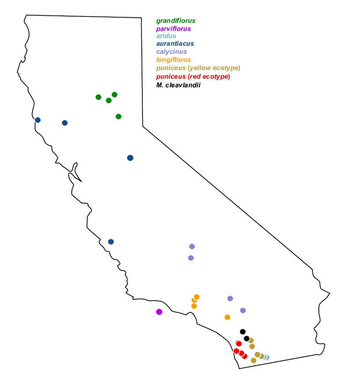
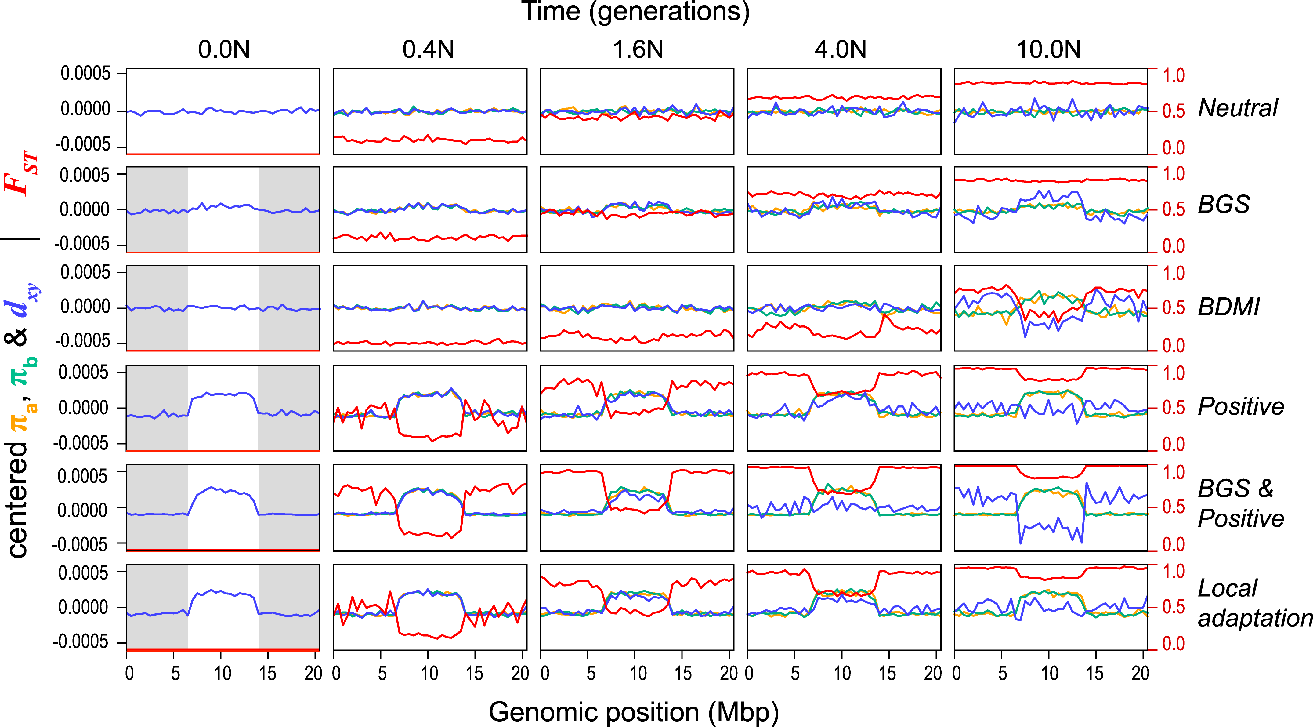
Monkeyflower (Mimulus aurantiacus) radiation in California shows wide adaptive range and phenotypic diversity. Stankowski et al. (2019) et al use simulations (SLiM and msprime) to shed light on processes that shape genomic landscapes, which are correlated between species.

We will look more closely at this system tomorrow.

Simulations are based on variations of a neutral base model that starts out with an ancestral population (N=10,000) that after 10N generation splits to two daughter populations (N=10,000 each) and are simulated another 10N generations. The chromosome is 21Mbp (similar in size to a monkeyflower chromosome) consisting of a central neutrally evolving region flanked by two regions where non-neutral processes are “allowed”. Models are:

1. neutral
2. BGS (non-neutral mutations are deleterious)
3. Bateson-Dobzhansky-Muller incompatibility (BDMI); after split, fraction variants deleterious in one population, neutral in other
4. positive selection
5. BGS and positive selection
6. local adaptation; 4 but also after split some variants beneficial in one population, neutral in other

Figure caption:

Fig 7. Genomic landscapes simulated under different divergence histories. Each row of plots shows patterns of within- and between-population variation (π, dxy, and FST) across the chromosome (500-kb windows) at 5 time points (N generations, where N = 10,000) during one of the scenarios The selection parameter (Ns, where s = Ns/N), proportion of deleterious (−) and positive mutations (+), and number of migrants per generation (Nm; 0 unless stated) for these simulations are as follows: (i) neutral divergence (no selection), (ii) BGS (−Ns = 100; −prop = 0.1), (iii) BDMI (−Ns = 100, −prop = 0.05, Nm = 0.1), (iv) positive selection (+Ns = 100, +prop = 0.001), (v) BGS and positive selection (−Ns = 100, −prop = 0.1; +Ns = 100, +prop = 0.005), and (vi) local adaptation (+Ns = 100, +prop = 0.001, Nm = 0.1). The gray boxes in the first column show the areas of the chromosome that are experiencing selection, while the white central area evolves neutrally. Note that π (in populations a and b) and dxy have been mean centered so they can be viewed on the same scale. Uncentered values and additional simulations with different parameter combinations and more time points can be found in S13 Fig. BDMI, Bateson-Dobzhansky-Muller incompatibility; BGS, background selection.

Neural network recombination landscape prediction

Figure 15: Cartoon of Recombination Landscape Estimation using Recurrent Neural Networks (ReLERNN) workflow (Adrion et al., 2020)

Use msprime simulations to generate training data for neural network.

Methods paper; one of the first examples of using msprime simulations to generate training data for a neural network.

Figure caption:

A cartoon depicting a typical workflow using ReLERNN’s four modules (shaded boxes) for (A) individually sequenced genomes or (B) pooled sequences. ReLERNN can optionally (dotted lines) utilize output from stairwayplot, SMC++, and MSMC to simulate under a demographic history with msprime. Training inlays show the network architectures used, with the GRU inlay in (B) depicting the gated connections within each hidden unit. Here, r, z, ht, and ht˜ are the reset gate, update gate, activation, and candidate activation, respectively (Cho et al. 2014). The genotype matrix encodes alleles as reference (−1), alternative (1), or padded/missing data (0; not shown). Variant positions are encoded along the real number line (0–1).

Bibliography

Adrion, J. R., Galloway, J. G., & Kern, A. D. (2020). Predicting the Landscape of Recombination Using Deep Learning. Molecular Biology and Evolution, 37(6), 1790–1808. https://doi.org/10.1093/molbev/msaa038

Baumdicker, F., Bisschop, G., Goldstein, D., Gower, G., Ragsdale, A. P., Tsambos, G., Zhu, S., Eldon, B., Ellerman, E. C., Galloway, J. G., Gladstein, A. L., Gorjanc, G., Guo, B., Jeffery, B., Kretzschumar, W. W., Lohse, K., Matschiner, M., Nelson, D., Pope, N. S., … Kelleher, J. (2022). Efficient ancestry and mutation simulation with msprime 1.0. Genetics, 220(3), iyab229. https://doi.org/10.1093/genetics/iyab229

DeGiorgio, M., Huber, C. D., Hubisz, M. J., Hellmann, I., & Nielsen, R. (2016). SweepFinder2: Increased sensitivity, robustness and flexibility. Bioinformatics, 32(12), 1895–1897. https://doi.org/10.1093/bioinformatics/btw051

Hahn, M. (2019). Molecular Population Genetics (First). Oxford University Press.

Haller, B. C., & Messer, P. W. (2019). SLiM 3: Forward Genetic Simulations Beyond the Wright. Molecular Biology and Evolution, 36(3), 632–637. https://doi.org/10.1093/molbev/msy228

Haller, B. C., & Messer, P. W. (2022). SLiM: An Evolutionary Simulation Framework.

Hein, J., Schierup, M. H., & Wiuf, C. (2005). Gene genealogies, variation and evolution: A primer in coalescent theory. Oxford University Press. https://books.google.se/books?id=CCmLNAEACAAJ

Kelleher, J., Wong, Y., Wohns, A. W., Fadil, C., Albers, P. K., & McVean, G. (2019). Inferring whole-genome histories in large population datasets. Nature Genetics, 51(9), 1330–1338. https://doi.org/10.1038/s41588-019-0483-y

Pope, N. S., Singh, A., Childers, A. K., Kapheim, K. M., Evans, J. D., & López-Uribe, M. M. (2023). The expansion of agriculture has shaped the recent evolutionary history of a specialized squash pollinator. Proceedings of the National Academy of Sciences, 120(15), e2208116120. https://doi.org/10.1073/pnas.2208116120

Stankowski, S., Chase, M. A., Fuiten, A. M., Rodrigues, M. F., Ralph, P. L., & Streisfeld, M. A. (2019). Widespread selection and gene flow shape the genomic landscape during a radiation of monkeyflowers. PLOS Biology, 17(7), e3000391. https://doi.org/10.1371/journal.pbio.3000391

Wakeley, J. (2008). Coalescent Theory: An Introduction (1st Edition edition). Roberts and Company Publishers.

Y. C. Brandt, D., Wei, X., Deng, Y., Vaughn, A. H., & Nielsen, R. (2022). Evaluation of methods for estimating coalescence times using ancestral recombination graphs. Genetics, iyac044. https://doi.org/10.1093/genetics/iyac044