Non-parametric rank based tests

Introduction

Hypothesis tests can be done via:

resampling (to obtain the null distribution)
using parametric tests (when the null distribution is known)
non-parametric rank based tests (derived before computers empowered statistics)

Non-parametric rank based test are useful when:

we do not know the underlying probability distribution and/or our data does not meet parametric test requirements
sample size is too small to properly assess the distribution of the data
transforming our data to meet the parametric test requirements would make interpretation of the results harder

Limitations

Some limitations of the non-parametric rank based tests include the facts that:

they are primary significance tests that often do not provide estimates of the effects of interest
they lead to waste of information and in consequence they have less power
when sample size are extremely small (e.g. $n=3$) rank tests cannot produce small P-values, even when the outcomes in the two groups are very different
non-parametric tests are less easily extended to situations where we wish to take into account the effect of more than one exposure on the outcome

Main non-parametric rank tests

Wilcoxon signed rank test
- compares the sample median against a hypothetical median (equivalent to one sample t-test)
- or examine the difference between paired observations (equivalent to paired t-test)
Wilcoxon rank sum test
- examines the difference between two unrelated groups
- equivalent to two sample t-test
Kruskal-Wallis one-way analysis of variance
- examines the difference between two or more unrelated groups
- equivalent to ANOVA

Rank based correlation

Spearman’s rank correlation
- Pearson’s correlation coefficient calculated on ranks

Kendall’s rank correlation
- based on number of concordant/discordant pairs
- alternative to Pearson correlation coefficient

Wilcoxon signed rank test

Named after Frank Wilcoxon (1892–1945), Wilcoxon signed rank test was one of the first “non-parametric” methods developed.

It can be used to:

compare the sample median against a hypothetical median (equivalent to one sample t-test)
examine the difference between paired observations (equivalent to paired t-test).

Wilcoxon signed rank test

for a median

Example 1 (Wilcoxon signed rank test (for a median)) Let’s imagine we are a part of team analyzing results of a placebo-controlled clinical trial to test the effectiveness of a sleeping drug. We have collected data on 10 patients when they took a sleeping drug and when they took a placebo.

The hours of sleep recorded for each study participant:

id	drug	placebo
1	6.1	5.2
2	6.0	7.9
3	8.2	3.9
4	7.6	4.7
5	6.5	5.3
6	5.4	7.4
7	6.9	4.2
8	6.7	6.1
9	7.4	3.8
10	5.8	7.3

Before we investigate the effect of drug, a senior statistician ask us:

“Is the median sleeping time without taking the drug significantly less than the recommended 7 h of sleep?”

Wilcoxon signed rank test

for a median (cont.)

Define the null and alternative hypothesis under the study

$H_0: m = m_0$ the median sleeping time is equal to $m_0$, $m_0 = 7$ h
$H_1 < m_0$ the median sleeping time is less than $m_0$, $m_0 = 7$ h

Calculate the value of the test statistics

we subtract the median from each measurement, $X_i - m_0$
we find absolute value of the difference, $|X_i - m_0|$
we rank the absolute value of the difference
we find the value of $W$, the Wilcoxon signed-rank test statistics as \[W =\displaystyle \sum_{i=1}^{n}Z_iR_i\] where $Z_i$ is an indicator variable such as:

\[\begin{equation} Z_i = \left\{ \begin{array}{cc} 0 & \mathrm{if\ } X_i - m_0 < 0 \\ 1 & otherwise \\ \end{array} \right. \end{equation}\]

Table 1: Demonstrating steps in the calculating W, Wilcoxon signed-rank test statistics on the placebo column: x stands for placebo sleeping hours
id	x	x-m0	abs(x-m0)	R	Z	ZR
1	5.2	-1.8	1.8	6.0	0	0.0
2	7.9	0.9	0.9	3.5	1	3.5
3	3.9	-3.1	3.1	9.0	0	0.0
4	4.7	-2.3	2.3	7.0	0	0.0
5	5.3	-1.7	1.7	5.0	0	0.0
6	7.4	0.4	0.4	2.0	1	2.0
7	4.2	-2.8	2.8	8.0	0	0.0
8	6.1	-0.9	0.9	3.5	0	0.0
9	3.8	-3.2	3.2	10.0	0	0.0
10	7.3	0.3	0.3	1.0	1	1.0
Note:
W = 6.5

Wilcoxon signed rank test

for a median (cont.)

Compare the value to the test statistics to values from known probability distribution

we got $W = 6.5$ and now we need to calculate the P-value associated with $W$ to be able to make decision about rejecting the null hypothesis.
we refer to a statistical table “Upper and Lower Percentiles of the Wilcoxon Signed Rank Test, W” that can be found online or here.
we can see, at sample size $n=10$, that observing a P-value associated with observing $W=6.5$ is just under $0.019$
assuming 5% significance level, we have enough evidence to reject the null hypothesis and conclude that the median is significantly less than 7 hours.

Wilcoxon signed rank test

for a median (cont.)

Where did that known distribution come from?

Wilcoxon described and showed examples how to calculate both the test statistics $W$ for an example data as well as the distribution of $W$ under the null hypothesis Wilcoxon (1945)
Let’s try to find the distribution of W assuming we only have four observation ($n=4$)

Wilcoxon signed rank test

for a median (cont.)…Where did that known distribution come from?

	c1	c2	c3	c4	c5	c6	c7	c8	c9	c10	c11	c12	c13	c14	c15	c16
id1	1	-1	1	1	1	-1	-1	-1	1	1	1	-1	-1	-1	1	-1
id4	2	2	-2	2	2	-2	2	2	-2	2	-2	-2	-2	2	-2	-2
id3	3	3	3	-3	3	3	-3	3	-3	-3	3	-3	3	-3	-3	-3
id4	4	4	4	4	-4	4	4	-4	4	-4	-4	4	-4	-4	-4	-4
W	10	9	8	7	6	7	6	5	5	3	4	4	3	2	1	0

Given 4 observations, we could get ranks $R_i$ of 1, 2, 3 or 4 only. Further, depending where the observation would be with respect to $m_0$, the rank $R_i$ could be positive or negative. For example, the first column $c1$ corresponds to all 4 observations having positive ranks, so all $x_i - m_0 > 0$, whereas column $c16$ corresponds to all observations having negative ranks, so $x_i - m_0 < 0$.

As $W$ test statistics is derived by summing up the positive ranks, we can see by listing all the combinations in the table, that $0 \le W \le10$.

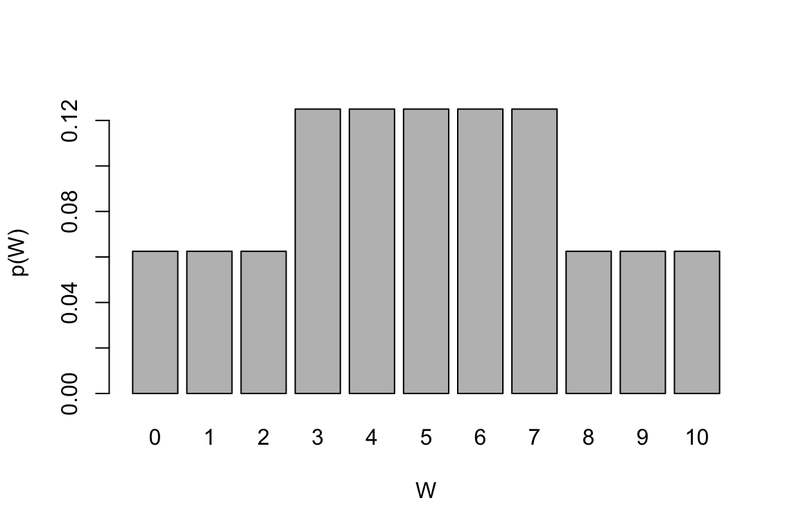
We can also write down the probability mass function

W	0	1	2	3	4	5	6	7	8	9	10
p(W)	0.0625	0.0625	0.0625	0.125	0.125	0.125	0.125	0.125	0.0625	0.0625	0.0625

And now we can use our knowledge from the Probability session on discrete distributions to calculate the probability of observed test statistics $W$ given the known probability mass function

Wilcoxon signed rank test

for a median (cont.)

In R we use wilcox.test() function:

# run Wilcoxon signed rank test for a median
wilcox.test(x = data.sleep$placebo, 
            y = NULL,
            alternative = "less",
            mu = 7,
            paired = FALSE)


    Wilcoxon signed rank test with continuity correction

data:  data.sleep$placebo
V = 6.5, p-value = 0.01827
alternative hypothesis: true location is less than 7

Wilcoxon signed rank test

paired observations

Example 2 (Wilcoxon signed rank test (paired observations)) Let’s return to our placebo-controlled clinical trial to test the effectiveness of a sleeping drug. Again, the hours of sleep we recorded for each participants are:

The hours of sleep recorded for each study participant:

id	drug	placebo
1	6.1	5.2
2	6.0	7.9
3	8.2	3.9
4	7.6	4.7
5	6.5	5.3
6	5.4	7.4
7	6.9	4.2
8	6.7	6.1
9	7.4	3.8
10	5.8	7.3

Is there enough evidence to reject a null hypothesis of the median of the differences between the paired observations being equal to 0? I.e. is the drug having an effect?

Wilcoxon signed rank test

paired observations

Define the null and alternative hypothesis under the study

$H_0:$ the median difference in the population equals to zero
$H_1:$ the median difference in the population does not equals to zero

Wilcoxon signed rank test

paired observations

To calculate test statistics:

calculate difference and exclude differences that equal to 0
rank difference in ascending order, ignoring the sign, e.g. the smallest difference value, here 0.6 is ranked 1.
sum up the ranks of the negative differences and of positive differences and denote these sums by $T_{-}$ and $T_{+}$ respectively
Why? If there were no differences in effectiveness between the sleeping drug and the placebo then the sums $T_{-}$ and $T_{+}$ would be similar. If there were a difference then one sum would be much smaller and one sum would be much larger than expected.
we get $T_{-} = 40$ and $T_{+} = 15$
denote the smaller sum by T and interpret the P-value, here $T = 15$

Table 2: Demonstrating steps in the calculating W, Wilcoxon signed-rank test statistics for difference in mean (paired observations)
id	drug	placebo	diff	rank
1	6.1	5.2	0.9	2
2	6.0	7.9	-1.9	5
3	8.2	3.9	4.3	10
4	7.6	4.7	2.9	8
5	6.5	5.3	1.2	3
6	5.4	7.4	-2.0	6
7	6.9	4.2	2.7	7
8	6.7	6.1	0.6	1
9	7.4	3.8	3.6	9
10	5.8	7.3	-1.5	4
Note:
T(-)=40$ , T(+) = 15

Wilcoxon signed rank test

paired observations

The “Critical values for the Wilcoxon matched pairs signed rank test” table can be found online or here
The Wilcoxon signed rank test is based on assessing whether $T$, the smaller of $T_{-}$ and $T_{+}$, is smaller than would be expected by chance, under the null hypothesis that the median of the paired differences is zero.
The hypothesis is that $T$ is equal to the sum of the ranks divided by 2, so that the smaller $T$ the more evidence there is against the null hypothesis.
Having our $T$ value we can check what is the probability of observing the value of $T$ under the null hypothesis, by checking the statistical table of “Critical values for the Wilcoxon matched pairs signed rank test”.
In our example, the sample size $n=10$, where $n$ is the number of non-zero differences (we had none) and 5% percentage point is 8. Since $T=15 > 8$ our $P-value > 0.05$ and we do not have enough evidence to reject the null hypothesis. There is no evidence of the sleeping drug working.

Wilcoxon signed rank test

paired observations

In R we use wilcox.test() function adjusting paired argument.

Before, Wilcoxon signed rank test for a median

# run Wilcoxon signed rank test for a median
wilcox.test(x = data.sleep$placebo, 
            y = NULL,
            alternative = "less",
            mu = 7,
            paired = FALSE)

Now, Wilcoxon signed rank test for paired observations

# run Wilcoxon signed rank test for paired observations 
wilcox.test(x = data.sleep$placebo, 
            y = data.sleep$drug,
            alternative = "two.sided",
            mu = 0,
            paired = TRUE)


    Wilcoxon signed rank test with continuity correction

data:  data.sleep$placebo and data.sleep$drug
V = 15, p-value = 0.2213
alternative hypothesis: true location shift is not equal to 0

2 or more unrelated groups

Wilcoxon rank sum test & Krusall-Wallis

Wilcoxon rank sum test

test statistics, $T$, is the sum or ranks in the smaller group
refer to table “Critical range for the Wilcoxon rank sum test” found online or here

Kruskall-Wallis

can be seen as extension of Wilcoxon rank sum test to $k≥2$ groups
for $k=2$ gives the same results as Wilcoxon rank sum test
the sums of the ranks in each of the $k$ groups should be comparable after allowing for any differences in sample size.

More details and examples in the chapter.

id	weight	smoking	rank
1	3.99	No	11
2	3.89	No	10
3	3.60	No	8
4	3.73	No	9
5	3.31	No	7
6	3.18	Yes	5
7	2.74	Yes	2
8	2.90	Yes	3
9	3.27	Yes	6
10	3.15	Yes	4
11	2.42	Yes	1

Correlation

Pearson correleation coefficient

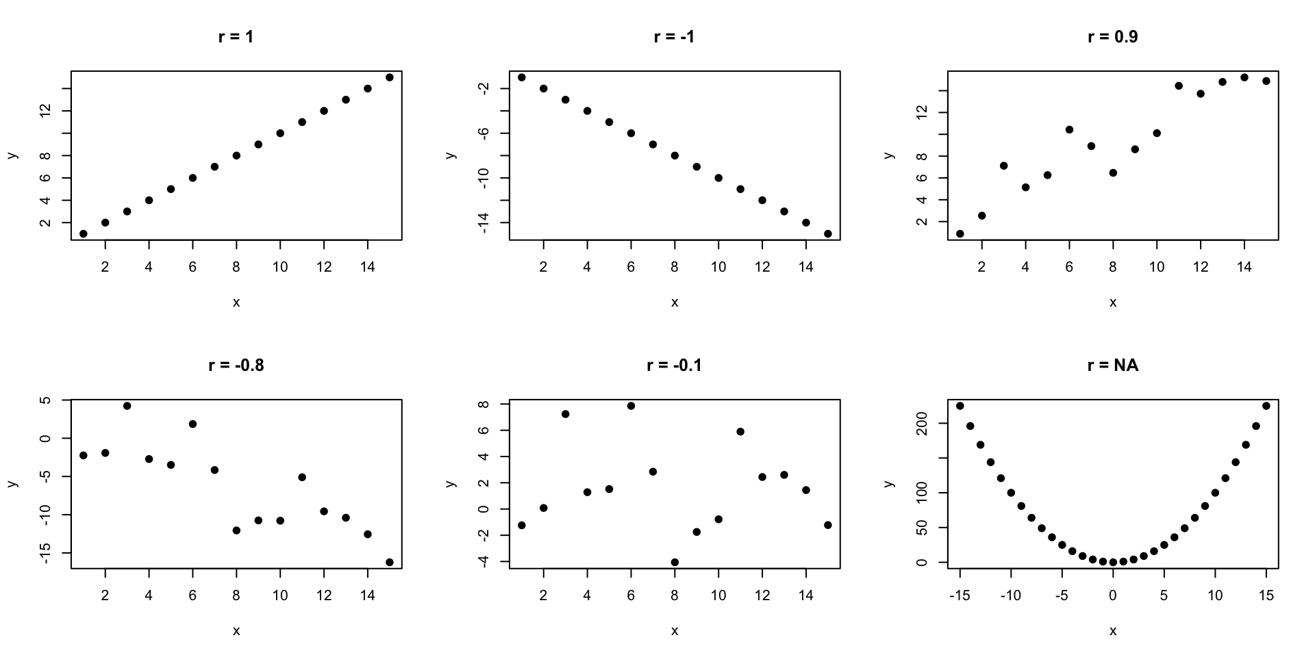
Pearson correlation coefficient, or rather more correctly Pearson product moment correlation coefficient, gives us an idea about the strength of association between two numerical variables. Its true value in the population, $\rho$, is estimated in the sample by $r$, where:

\[r=\frac{\sum(x-\bar{x})(x-\bar{y})}{\sqrt{\sum(x-\bar{x})^2\sum(x-\bar{y})^2}} \qquad(1)\]

Spearman and Kendal tau

Spearman’s rank correlation

To calculate Spearman’s rank correlation between two variables $X$ and $Y$ we:

rank the values of $X$ and $Y$ independently

follow the formula to calculate the Pearson correlation coefficient using ranks

Kendall’s tau

To calculate Kendall’s tau, $\tau$, we compare ranks of $X$ and $Y$ between every pair of observation. (There are n(n-1)/2 possible pairs). The pairs of ranks for observation $i$ and $j$ are said to be:

concordant: if they differ in the same direction, i.e. if both the $X$ and $Y$ ranks of subject $i$ are lower than the corresponding ranks of subject $j$, or both are higher
discordant: otherwise

\[\tau = \frac{n_C-n_D}{n(n-1)/2}\] where

$n_C$, number of concordant pairs $n_D$, number of discordant pairs

Kendall $\tau$

Although Spearman correlation coefficient is commonly used it may be easier to build intuitive understanding of Kendall $\tau$. A positive correlation indicates that the ranks of both variables increase together whilst a negative correlation indicates that as the rank of one variable increases the other one decreases

Summary

Non-parametric rank based tests still have their place in modern data analysis
They are based on a neat idea of turning data into ranks that is useful when sample is small or when parametric based test assumptions cannot be met
Spearman correlation is perhaps used as a first choice when Pearson correlation coefficient should not be calculated. However Kendall tau’s offers much easier interpretation, with positive correlation indicating that the ranks of both variables increase together

References

Wilcoxon, Frank. 1945. “Individual Comparisions by Ranking Methods.” Biometrics Bulletin 1 (6): 80–83.

Thank you for listening

Any questions?

id	drug	placebo
1	6.1	5.2
2	6.0	7.9
3	8.2	3.9
4	7.6	4.7
5	6.5	5.3
6	5.4	7.4
7	6.9	4.2
8	6.7	6.1
9	7.4	3.8
10	5.8	7.3

	c1	c2	c3	c4	c5	c6	c7	c8	c9	c10	c11	c12	c13	c14	c15	c16
id1	1	-1	1	1	1	-1	-1	-1	1	1	1	-1	-1	-1	1	-1
id4	2	2	-2	2	2	-2	2	2	-2	2	-2	-2	-2	2	-2	-2
id3	3	3	3	-3	3	3	-3	3	-3	-3	3	-3	3	-3	-3	-3
id4	4	4	4	4	-4	4	4	-4	4	-4	-4	4	-4	-4	-4	-4
W	10	9	8	7	6	7	6	5	5	3	4	4	3	2	1	0

id	drug	placebo
1	6.1	5.2
2	6.0	7.9
3	8.2	3.9
4	7.6	4.7
5	6.5	5.3
6	5.4	7.4
7	6.9	4.2
8	6.7	6.1
9	7.4	3.8
10	5.8	7.3

id	drug	placebo
1	6.1	5.2
2	6.0	7.9
3	8.2	3.9
4	7.6	4.7
5	6.5	5.3
6	5.4	7.4
7	6.9	4.2
8	6.7	6.1
9	7.4	3.8
10	5.8	7.3

	c1	c2	c3	c4	c5	c6	c7	c8	c9	c10	c11	c12	c13	c14	c15	c16
id1	1	-1	1	1	1	-1	-1	-1	1	1	1	-1	-1	-1	1	-1
id4	2	2	-2	2	2	-2	2	2	-2	2	-2	-2	-2	2	-2	-2
id3	3	3	3	-3	3	3	-3	3	-3	-3	3	-3	3	-3	-3	-3
id4	4	4	4	4	-4	4	4	-4	4	-4	-4	4	-4	-4	-4	-4
W	10	9	8	7	6	7	6	5	5	3	4	4	3	2	1	0

id	drug	placebo
1	6.1	5.2
2	6.0	7.9
3	8.2	3.9
4	7.6	4.7
5	6.5	5.3
6	5.4	7.4
7	6.9	4.2
8	6.7	6.1
9	7.4	3.8
10	5.8	7.3

id	drug	placebo
1	6.1	5.2
2	6.0	7.9
3	8.2	3.9
4	7.6	4.7
5	6.5	5.3
6	5.4	7.4
7	6.9	4.2
8	6.7	6.1
9	7.4	3.8
10	5.8	7.3

	c1	c2	c3	c4	c5	c6	c7	c8	c9	c10	c11	c12	c13	c14	c15	c16
id1	1	-1	1	1	1	-1	-1	-1	1	1	1	-1	-1	-1	1	-1
id4	2	2	-2	2	2	-2	2	2	-2	2	-2	-2	-2	2	-2	-2
id3	3	3	3	-3	3	3	-3	3	-3	-3	3	-3	3	-3	-3	-3
id4	4	4	4	4	-4	4	4	-4	4	-4	-4	4	-4	-4	-4	-4
W	10	9	8	7	6	7	6	5	5	3	4	4	3	2	1	0

id	drug	placebo
1	6.1	5.2
2	6.0	7.9
3	8.2	3.9
4	7.6	4.7
5	6.5	5.3
6	5.4	7.4
7	6.9	4.2
8	6.7	6.1
9	7.4	3.8
10	5.8	7.3