suppressPackageStartupMessages({
  library(TFBSTools)
  library(Biostrings)
  library(JASPAR2024)
  library(RSQLite)
  library(BSgenome.Mmusculus.UCSC.mm39)
  library(TxDb.Mmusculus.UCSC.mm39.knownGene)
  library(GenomicRanges)
  library(monaLisa)
})

# ## To install the latest tool versions, and from the current bioconductor release (3.21)
# pkgs <- c("TFBSTools", "Biostrings", "JASPAR2024", "RSQLite",
#           "BSgenome.Mmusculus.UCSC.mm39", "TxDb.Mmusculus.UCSC.mm39.knownGene",
#           "GenomicRanges", "monaLisa")
# bioc <- "3.21" # with R 4.5
# #libPath <- "/path/to/custom/folder/if/desired"
# BiocManager::install(pkgs = pkgs,
#                      update = TRUE,
#                      ask = TRUE,
#                      checkBuilt = FALSE,
#                      force = FALSE,
#                      # lib = libPath,
#                      version = bioc)

# ## if you need to install a specific version of a package you can do so as follows
# remotes::install_version("ggplot2", version = "3.5.2")1 Background
DNA-binding proteins, called transcription factors (TFs), play key roles in gene expression regulation, including the regulation of cellular functions and during organismal development. The TF binding sites (TFBSs) tend to be in the range of 6-12 base pairs (bp) long (Spitz and Furlong, 2012). The effect of their binding can be indirectly observed via associated changes in transcription, chromatin accessibility, DNA methylation and histone modifications.
Here, we will examine how the TFBSs, also called motifs, can be represented in the form of nucleotide (rows) x position (columns) matrices, such as the position weight matrix (PWM). We will learn how such matrices can be created, downloaded from public databases like Jaspar, and use them to scan against a reference sequence in search for predicted motif hits.
2 Learning outcomes
- Understand how motifs can be represented in nucleotide x sequence position matrices.
- Understand the differences between the position frequency matrix (PFM), position probability matrix (PPM), position weight matrix (PWM), and information content matrix (ICM), and learn how these matrices can be constructed.
- Learn how to load PWMs in
Rand scan for motif hits against a reference.
3 Libraries
We start by loading the needed packages. If necessary, use BiocManager::install() to install missing packages. Note that we will need to work with the latest version of monaLisa if using ggplo2>=4.0.0.
4 Motif databases
As mentioned, TFBSs or motifs can be represented in matrices with rows corresponding to the nucleotides, namely \(A\), \(C\), \(G\), and \(T\), and columns corresponding to the position along the binding site. The position frequency matrix (PFM), also called the position count matrix (PCM), shows the count each nucleotide contributes at a particular position. Such matrices can be obtained from publicly available databases like Jaspar (Sandelin et al.) and Hocomoco (Vorontsov, Eliseeva, Zinkevich, et al.). In this tutorial we will focus on Jaspar, which is also available as Bioconductor packages like JASPAR2024.
Jaspar is an open-access database that provides TF binding preferences in the form of position frequency matrices (PFMs). PFMs are generated by aligning DNA binding-site sequences from high-quality experiments such as ChIP-seq, protein binding microarrays, and SELEX-based methods, along with incorporating curated external motifs. More details about this can be found on the Jaspar website.
5 Position frequency matrix
As stated, the PFM depicts the frequencies of the nucleotides i.e. the number of times each nucleotide occurs at each position along the motif. Note that the motif positions are independent of one another in this representation.
To illustrate this more we will use the CTCFL motif as an example by reading in the DNA sequences which we have downloaded from Jaspar and producing the corresponding PFM. We will use the Biostrings package to read the sequences and represent them as a DNAStringSet object, which is a convenient way to represent and manipulate DNA sequences in R. See the vignette from the Biostrings package for more details.
Let’s set up our working directory and download the data.
# go to your working directory and make a data folder
mkdir data

# option A: download the file from Jaspar
wget -P data https://jaspar.elixir.no/download/data/2024/sites/MA1102.3.sites

# option B: download the file from GitHub
wget -P data https://github.com/NBISweden/workshop-epigenomics-RTDs/blob/master/docs/content/tutorials/motifAnalyses/data/MA1102.3.sites
# read in the TFBS sequences
CTCFLsequencesFile <- "data/MA1102.3.sites"
CTCFLsequences <- readDNAStringSet(CTCFLsequencesFile)
CTCFLsequencesDNAStringSet object of length 18037:
width seq names
[1] 8 CAGGGGGC hg38_chr1:869925-...
[2] 8 CAGGGGGC hg38_chr1:904775-...
[3] 8 GAGGGGGC hg38_chr1:925040-...
[4] 8 CAGGGGGC hg38_chr1:945418-...
[5] 8 GAGGGGGC hg38_chr1:951563-...
... ... ...
[18033] 8 AAGGGGGC hg38_chrX:1550575...
[18034] 8 GAGGGGGC hg38_chrX:1552166...
[18035] 8 CAGGGGGA hg38_chrX:1552168...
[18036] 8 CAGGGGGC hg38_chrX:1554355...
[18037] 8 GAGGGGGC hg38_chrX:1556122...We can see that we have a total of 18037 sequences of the TF binding site. Next, we generate the PFM by counting the nucleotide occurrences per position.
# create PFM by counting nucleotide occurrences per position
pfm <- consensusMatrix(CTCFLsequences)
pfm <- pfm[c("A", "C", "G", "T"), ]
pfm
[,1] [,2] [,3] [,4] [,5] [,6] [,7] [,8]
A 1301 17270 86 684 349 193 351 181
C 12867 413 481 600 1141 767 270 17593
G 2033 329 17285 16511 15425 16819 17001 68
T 1836 25 185 242 1122 258 415 1956 Position probability matrix
We can now calculate the probability of observing each nucleotide at a particular position by dividing counts by the total count per position.
\[ PPM_{ij} = \frac{count_{ij}}{\sum_{i}{count_{ij}}} \]
Where \(i\) is the nucleotide and \(i \in \{A, C, G, T\}\), and \(j\) is the position along the motif.
# calculate PPM
ppm <- sweep(x = pfm, MARGIN = 2, STATS = colSums(pfm), FUN = "/")
ppm
[,1] [,2] [,3] [,4] [,5] [,6] [,7]
A 0.07212951 0.95747630 0.004767977 0.03792205 0.01934912 0.01070023 0.01946000
C 0.71336697 0.02289738 0.026667406 0.03326496 0.06325886 0.04252370 0.01496923
G 0.11271276 0.01824028 0.958307923 0.91539613 0.85518656 0.93247214 0.94256251
T 0.10179076 0.00138604 0.010256695 0.01341687 0.06220547 0.01430393 0.02300826
[,8]
A 0.010034928
C 0.975383933
G 0.003770028
T 0.010811110# all positions now sum to 1
colSums(ppm)[1] 1 1 1 1 1 1 1 1Now we can calculate the probability of observing a certain motif sequence by multiplying the probabilities of each nucleotide per position. Let us look at some examples below.
p_CAGACGGC <- ppm["C", 1] * ppm["A", 2] * ppm["G", 3] * ppm["A", 4] *
  ppm["C", 5] * ppm["G", 6] * ppm["G", 7] * ppm["C", 8]
p_CAGACGGC
C
0.001346111 p_AATTGGTT <- ppm["A", 1] * ppm["A", 2] * ppm["T", 3] * ppm["T", 4] *
ppm["G", 5] * ppm["G", 6] * ppm["T", 7] * ppm["T", 8]
p_AATTGGTT A
1.885169e-09 In this PPM, we do not have any zero counts for any given nculeotide and position. What would happen if we did? Let us suppose that pfm["T", 7] had a count of zero and therefore ppm["T", 7] is also zero. Multiplying by zero would result in p_AATTGGTT = 0. This issue can especially emerge when starting from a low number of sequences to construct the PFM. To avoid low count issues, we will add a peudo-count \(p\) of 1 per position, to the PFM. This corresponds to a pseudo-count of \(p/N\) for each entry in the matrix, where \(N\) is the total number of nucleotides, and \(N=4\) in our case. We will then re-calculate the PPM.
\[ PPM_{ij} = \frac{count_{ij}+\frac{p}{N}}{\sum_{i}{count_{ij}+p}} \]
# set p and N
pseudooCount <- 1
N <- nrow(pfm)

# add pseudo-count to PFM and re-calculate PPM
pfmWithPseudo <- pfm + pseudooCount/N
ppm <- sweep(x = pfmWithPseudo, MARGIN = 2, STATS = colSums(pfm), FUN = "/")
ppm
[,1] [,2] [,3] [,4] [,5] [,6] [,7]
A 0.07214337 0.95749016 0.004781837 0.03793591 0.01936298 0.01071409 0.01947386
C 0.71338083 0.02291124 0.026681266 0.03327882 0.06327272 0.04253756 0.01498309
G 0.11272662 0.01825414 0.958321783 0.91540999 0.85520042 0.93248600 0.94257637
T 0.10180462 0.00139990 0.010270555 0.01343073 0.06221933 0.01431779 0.02302212
[,8]
A 0.010048789
C 0.975397793
G 0.003783889
T 0.0108249717 Position weight matrix
The position weight matrix (PWM) is also known as the position-specific scoring matrix or the logodds scoring matrix. Here, log-odds scores are calculated by comparing the probabilities we have in the PPM to the probabilities of observing each nucleotide outside of a binding site (background nucleotide probabilities). Assuming a uniform background, in which each nucleotide has an equal probability, would give us the following background probabilities for each nucleotide: \(p(A) = p(C) = p(G) = p(T) = 0.25\). The log-odds scores can be obtained as follows:
\[ PWM_{ij}=log_2\Bigl(\frac{PPM_{ij}}{B_i}\Bigr) \]
Where \(i\) is the nucleotide, \(j\) is the position along the motif, and \(B_i\) is the background probability for nucleotide \(i\). Thanks to the pseudo-count we have added, we will avoid situations where we are taking the \(log_2(0)\) which is \(-Inf\).
# define background probabilities
(B <- c("A" = 0.25, "C" = 0.25, "G" = 0.25, "T" = 0.25))
A C G T
0.25 0.25 0.25 0.25 # calculate PWM
pwm <- log2(sweep(x = ppm, MARGIN = 2, STATS = B, FUN = "/"))
pwm [,1] [,2] [,3] [,4] [,5] [,6] [,7]
A -1.792989 1.937330 -5.708219 -2.720292 -3.690555 -4.544347 -3.682317
C 1.512744 -3.447801 -3.228029 -2.909252 -1.982273 -2.555119 -4.060521
G -1.149100 -3.775632 1.938582 1.872490 1.774334 1.899154 1.914681
T -1.296125 -7.480460 -4.605342 -4.218319 -2.006493 -4.126047 -3.440835
[,8]
A -4.636835
C 1.964063
G -6.045915
T -4.529493The score for a specific sequence can now be calculated by combining the PWM scores at each position. For example the score for CAGACGGC is:
pwm["C", 1] + pwm["A", 2] + pwm["G", 3] + pwm["A", 4] + pwm["C", 5] + pwm["G", 6]+ pwm["G", 7] + pwm["C", 8] C
6.463989 In this manner, PWMs can be used to scan for motif matches against a reference DNA sequence. The matchPWM function from the Biostrings can be used to do that. Matches with scores greater that the set min.score will be called as predicted binding sites. min.score can be set as a fixed empiric number or as a character reflecting the percentage of the highest possible score. See the matchPWM function for more details. Let us try scanning for this motif against a given DNA string.
# reference DNA sequence (this is typically the reference genome)
refDNA <-"GCCTATACAGACGGCGTTGGATATACGCAGACGGCTGTGA"
matchPWM(pwm, subject = refDNA, min.score = 6)Views on a 40-letter DNAString subject
subject: GCCTATACAGACGGCGTTGGATATACGCAGACGGCTGTGA
views:
start end width
[1] 8 15 8 [CAGACGGC]
[2] 28 35 8 [CAGACGGC]
TipExercise
Using the PWM we have created, calculate the score for sequence CAGGGGGC. Then, using the matchPWM function and setting min.score=10, find the motif matches in the following reference sequence: GGCAGGGGGCTGCCCCGACAGACGGCCTAGGTATGCTGTTCCCACAGGGGGCTCTTCCGGGGTGTCAGGGGGCTT.
Show solution
# reference DNA sequence (this is typically the reference genome)
refDNA <- "GGCAGGGGGCTGCCCCGACAGACGGCCTAGGTATGCTGTTCCCACAGGGGGCTCTTCCGGGGTGTCAGGGGGCTT"
matchPWM(pwm, subject = refDNA, min.score = 10)Views on a 75-letter DNAString subject
subject: GGCAGGGGGCTGCCCCGACAGACGGCCTAGGTAT...CCACAGGGGGCTCTTCCGGGGTGTCAGGGGGCTT
views:
start end width
[1] 3 10 8 [CAGGGGGC]
[2] 45 52 8 [CAGGGGGC]
[3] 66 73 8 [CAGGGGGC]
8 Information content matrix
The information content matrix (ICM) can additionally reflect which positions along the motif are more or less conserved. To have a better understanding of this, we need to first introduce some key concepts in information theory, a field established by Claude Shannon with his influential publication in 1948, entitled “A Mathematical Theory of Communication”. We will largely borrow explanations from David McKay’s book “Information Theory, Inference, and Learning Algorithms”, which offers great explanations and deeper dives into the topic for those interested.
Let us consider a random variable \(X\) with an outcome \(x\). The Shannon information content of \(x\) is defined as \(h(x)=log_2\frac{1}{p(x)}\), where \(p(x)\) is the probability of outcome \(x\). It is measured in bits since we are using \(log_2\), and reflects a measure of surprise from an outcome. For example, an outcome with probability of 1 is not very surprising and thus provides no information if observed: \(log_2(1)=0\). Whereas an outcome with a very low probability is more surprising and provides more information were it to happen. For example, assume the following probabilities of observing the outcome of a random variable \(X\): \(p(x=0)=0.4\) and \(p(x=1)=0.6\). You could imagine a bent coin with binary outcomes. The Shannon information content for outcome \(x=0\) is \(h(x=0)=log_2\frac{1}{p(x=0)}=log_2\frac{1}{0.4}\approx1.322\).
The entropy represents the average Shannon information content of an outcome and is: \[ H(X)=\sum_{x}p(x)log_2\frac{1}{p(x)} \]
Following our example from above, the entropy of \(X\) is \[ \begin{aligned} H(X) &= \sum_{x}p(x)log_2\frac{1}{p(x)} \\ &= p(x=0)log_2\frac{1}{p(x=0)} + p(x=1)log_2\frac{1}{p(x=1)} \\ &= 0.4log_2\frac{1}{0.4} + 0.6log_2\frac{1}{0.6} \\ &\approx 0.971 \end{aligned} \]
We can think of it as an average measure of surprise. Another name for the entropy is the uncertainty. You may notice that it is maximized when we have uniform probabilities.
Coming back to our motif, we want to calculate the bits per position, and use that to reflect the degree of conservation of the positions. We calculate this by taking the maximum uncertainty per position and subtracting the actual uncertainty at that position. As mentioned, uncertainty (entropy) is maximum when all outcomes have equal probabilities. In our case, the outcome is the specific instance of a nucleotide. We thus have 4 outcomes (\(A\), \(C\), \(G\), and \(T\)). In a scenario, where all nucleotides are equally likely, there is no preference for any particular nucleotide. Assuming equal probabilities of \(\frac{1}{N}\) for each nucleotide, where \(N\) is the total number of nucleotides, the maximum entropy, or total information content \(IC_{total}\), can be calculated as follows: \[ \begin{aligned} IC_{total} &= \sum_{x}p(x)log_2\frac{1}{p(x)} \\ &= N*\frac{1}{N}log_2N \\ &= log_2N \\ &= log_24 \\ &= 2 \end{aligned} \]
The actual uncertainty \(U\) per position is \[ \begin{aligned} U &= \sum_{x}p(x)log_2\frac{1}{p(x)} \\ &= -\sum_{x}p(x)log_2p(x) \end{aligned} \] The final information content \(IC_{final}\) per position is: \[ \begin{aligned} IC_{final} &= IC_{total}-U \\ &= 2-U \end{aligned} \]
When \(U=0\) (when one nucleotide has a probability of 1), \(IC_{final}=2-0=2\) and you know the nucleotide with no uncertainty. This reflects a highly conserved nucleotide.
Following our example motif, let us calculate \(IC_{final}\) for each position.
# total information content (maximum uncertainty)
IC_total <- log2(4)
IC_total[1] 2# actual uncertainty per position
U <- -colSums(apply(X = ppm, MARGIN = 2, FUN = function(x){
x*log2(x)
}))
U [1] 1.3117860 0.3035231 0.3030486 0.5426832 0.8044259 0.4456293 0.4071408
[8] 0.2028718# final information content per position
IC_final <- IC_total - U
IC_final[1] 0.688214 1.696477 1.696951 1.457317 1.195574 1.554371 1.592859 1.797128Finally, to get the ICM where the height of each nulceotide (letter) shows the bits each nucleotide contributes, we will multiply the probability of each nucleotide by \(IC_{final}\) per position.
# ICM
icm <- sweep(x = ppm, MARGIN = 2, STATS = IC_final, FUN = "*")
icm [,1] [,2] [,3] [,4] [,5] [,6]
A 0.04965008 1.624359931 0.008114546 0.05528464 0.02314987 0.01665366
C 0.49095866 0.038868386 0.045276813 0.04849778 0.07564722 0.06611914
G 0.07758003 0.030967734 1.626225532 1.33404237 1.02245549 1.44942889
T 0.07006336 0.002374898 0.017428633 0.01957282 0.07438782 0.02225515
[,7] [,8]
A 0.03101912 0.018058961
C 0.02386595 1.752914869
G 1.50139141 0.006800133
T 0.03667100 0.019453860# create ICMatrix object to use the seqLogo function from TFBSTools
icmatrix <- ICMatrix(ID = "MA1102.3",
name = "CTCFL",
profileMatrix = icm)
icmatrixAn object of class ICMatrix
ID: MA1102.3
Name: CTCFL
Matrix Class: Unknown
strand: +
Pseudocounts:
Schneider correction:
Tags:
list()
Background:
   A    C    G    T
0.25 0.25 0.25 0.25
Matrix:
        [,1]        [,2]        [,3]       [,4]       [,5]       [,6]
A 0.04965008 1.624359931 0.008114546 0.05528464 0.02314987 0.01665366
C 0.49095866 0.038868386 0.045276813 0.04849778 0.07564722 0.06611914
G 0.07758003 0.030967734 1.626225532 1.33404237 1.02245549 1.44942889
T 0.07006336 0.002374898 0.017428633 0.01957282 0.07438782 0.02225515
        [,7]        [,8]
A 0.03101912 0.018058961
C 0.02386595 1.752914869
G 1.50139141 0.006800133
T 0.03667100 0.019453860
# draw motif sequence logo
seqLogo(icmatrix)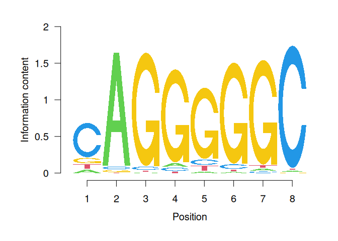
This is a useful way to visualize motifs, and get a sense of how conserved the sequence is at each position.
9 Scanning for motif hits
Now that we have a good understanding of the PWM and the other matrices, let us see how we can load a list of PWMs from Jaspar and what useful functions are at our disposal. We will extract the list of all vertebrate TFs.
# extract PFMs of vertebrate TFs from JASPAR2024
JASPAR2024 <- JASPAR2024()
JASPARConnect <- RSQLite::dbConnect(RSQLite::SQLite(), db(JASPAR2024))
pfmList <- TFBSTools::getMatrixSet(JASPARConnect,
                                   opts = list(tax_group = "vertebrates",
                                               collection="CORE",
                                               matrixtype = "PFM")
)
pfmList
PFMatrixList of length 879
names(879): MA0004.1 MA0069.1 MA0071.1 MA0074.1 ... MA1721.2 MA1602.2 MA1722.2pfmList[[1]]An object of class PFMatrix
ID: MA0004.1
Name: Arnt
Matrix Class: Basic helix-loop-helix factors (bHLH)
strand: +
Tags:
$alias
[1] "HIF-1beta,bHLHe2"
$description
[1] "aryl hydrocarbon receptor nuclear translocator"
$family
[1] "PAS domain factors"
$medline
[1] "7592839"
$remap_tf_name
[1] "ARNT"
$symbol
[1] "ARNT"
$tax_group
[1] "vertebrates"
$tfbs_shape_id
[1] "11"
$type
[1] "SELEX"
$unibind
[1] "1"
$collection
[1] "CORE"
$species
10090
"Mus musculus"
$acc
[1] "P53762"
Background:
   A    C    G    T
0.25 0.25 0.25 0.25
Matrix:
[,1] [,2] [,3] [,4] [,5] [,6]
A 4 19 0 0 0 0
C 16 0 20 0 0 0
G 0 1 0 20 0 20
T 0 0 0 0 20 0# we can convert the PFMs to PWMs
pwmList <- toPWM(pfmList)
pwmList[[1]]@profileMatrix [,1] [,2] [,3] [,4] [,5] [,6]
A -0.3081223 1.884523 -4.700440 -4.700440 -4.700440 -4.700440
C 1.6394103 -4.700440 1.957772 -4.700440 -4.700440 -4.700440
G -4.7004397 -2.115477 -4.700440 1.957772 -4.700440 1.957772
T -4.7004397 -4.700440 -4.700440 -4.700440 1.957772 -4.700440# Alternatively, we can directly load the PWMs
pwmList <- TFBSTools::getMatrixSet(JASPARConnect,
opts = list(tax_group = "vertebrates",
collection="CORE",
matrixtype = "PWM")
)
pwmList[[1]]@profileMatrix [,1] [,2] [,3] [,4] [,5] [,6]
A -0.3081223 1.884523 -4.700440 -4.700440 -4.700440 -4.700440
C 1.6394103 -4.700440 1.957772 -4.700440 -4.700440 -4.700440
G -4.7004397 -2.115477 -4.700440 1.957772 -4.700440 1.957772
T -4.7004397 -4.700440 -4.700440 -4.700440 1.957772 -4.700440# pwmList is a PWMatrixList object
# we can look at the structure and information available for the first motif
str(pwmList[[1]])Formal class 'PWMatrix' [package "TFBSTools"] with 8 slots
..@ pseudocounts : num 0.8
..@ ID : chr "MA0004.1"
..@ name : chr "Arnt"
..@ matrixClass : chr "Basic helix-loop-helix factors (bHLH)"
..@ strand : chr "+"
..@ bg : Named num [1:4] 0.25 0.25 0.25 0.25
.. ..- attr(*, "names")= chr [1:4] "A" "C" "G" "T"
..@ tags :List of 13
.. ..$ alias : chr "HIF-1beta,bHLHe2"
.. ..$ description : chr "aryl hydrocarbon receptor nuclear translocator"
.. ..$ family : chr "PAS domain factors"
.. ..$ medline : chr "7592839"
.. ..$ remap_tf_name: chr "ARNT"
.. ..$ symbol : chr "ARNT"
.. ..$ tax_group : chr "vertebrates"
.. ..$ tfbs_shape_id: chr "11"
.. ..$ type : chr "SELEX"
.. ..$ unibind : chr "1"
.. ..$ collection : chr "CORE"
.. ..$ species : Named chr "Mus musculus"
.. .. ..- attr(*, "names")= chr "10090"
.. ..$ acc : chr "P53762"
..@ profileMatrix: num [1:4, 1:6] -0.308 1.639 -4.7 -4.7 1.885 ...
.. ..- attr(*, "dimnames")=List of 2
.. .. ..$ : chr [1:4] "A" "C" "G" "T"
.. .. ..$ : NULL# we can access some entries with the functions shown below on an example
# PWMatrix, but they can also be used on the PWMatrixList
motif <- pwmList[[1]]
# ... motif name
name(motif)[1] "Arnt"# ... motif ID
ID(motif)[1] "MA0004.1"# ... used background probabilities
bg(motif) A C G T
0.25 0.25 0.25 0.25 # ... motif tags
tags(motif)$alias
[1] "HIF-1beta,bHLHe2"
$description
[1] "aryl hydrocarbon receptor nuclear translocator"
$family
[1] "PAS domain factors"
$medline
[1] "7592839"
$remap_tf_name
[1] "ARNT"
$symbol
[1] "ARNT"
$tax_group
[1] "vertebrates"
$tfbs_shape_id
[1] "11"
$type
[1] "SELEX"
$unibind
[1] "1"
$collection
[1] "CORE"
$species
10090
"Mus musculus"
$acc
[1] "P53762"# disconnect Db
dbDisconnect(JASPARConnect)As we have seen, PWMs can be used to scan for potential TFBSs against a reference sequence. To illustrate this, let us use some of the PWMs we have loaded from Jaspar above, to scan against hits at the gene promoters from the UCSC mouse reference genome. We will use the findMotifHits function from the monaLisa package to scan for motif hits. This function uses Biostrings::matchPWM internally to scan for matches, but additionally allows for the subject argument to accept DNAStringSet or GRanges objects. It also allows for parallelization across PWMs with the BPPARAM argument.
# get promoters as GRanges object
promoters <- trim(promoters(TxDb.Mmusculus.UCSC.mm39.knownGene,
                       upstream = 1000, downstream = 500))

# extract promoter sequences
promoterSeqs <- getSeq(BSgenome.Mmusculus.UCSC.mm39, promoters)
promoterSeqs
DNAStringSet object of length 278369:
width seq names
[1] 1500 CCCTTTTGGATAGATTCTAGG...GATTTATGAGTAAGGGATGT ENSMUST00000193812.2
[2] 1500 TTCTGAGGAGAGTGGCTCATA...AGGTAGCAACAGATATGGCA ENSMUST00000082908.3
[3] 1500 GTCTACCACATAGTTGCACAT...GCAATAGAAATTTGTTAAAA ENSMUST00000192857.2
[4] 1500 ACTTAAACACTAAATATGCGG...TTCAAGGATGGCCATGAATT ENSMUST00000161581.3
[5] 1500 TGATTAAGAAAATTCCCTGGT...TTGGTGTGGTAGTCACGTCC ENSMUST00000192183.2
... ... ...
[278365] 1500 CATGCTGACACCCCAATGGGG...AACACTGCAGAAGATGGAGG ENSMUST00020182238.1
[278366] 1500 TGAGAACACTGCAGAAGATGG...ATTAAAGATTGTTTTTTCTC ENSMUST00020182428.1
[278367] 1500 TGACCTTGTAAAACTAGTGGG...AGGACCCTCTGGCCTGAAAG ENSMUST00000381725.1
[278368] 1500 TTCCAGGTCCTACCATGTGAG...TGTGTACACCAGGCTGGCCT ENSMUST00000179505.8
[278369] 1500 CGTTTTTCAGTTTTCTCACCA...TTTTTTTCGAGACTGGGTTT ENSMUST00000178343.2# choose first 5 PWM as an example
pwms <- pwmList[1:5]
name(pwms) MA0004.1 MA0069.1 MA0071.1 MA0074.1 MA0101.1
"Arnt" "PAX6" "RORA" "RXRA::VDR" "REL" # scan for motif hits with 4 cores
hits <- findMotifHits(query = pwms,
subject = promoterSeqs,
min.score = 10.0,
method = "matchPWM",
BPPARAM = BiocParallel::MulticoreParam(4))
hitsGRanges object with 504290 ranges and 4 metadata columns:
seqnames ranges strand | matchedSeq pwmid
<Rle> <IRanges> <Rle> | <DNAStringSet> <Rle>
[1] ENSMUST00000193812.2 915-924 - | TGGCATTTCC MA0101.1
[2] ENSMUST00000082908.3 768-781 - | TTTATGCATCATAT MA0069.1
[3] ENSMUST00000192857.2 1059-1072 - | TTAATGCATCAGTG MA0069.1
[4] ENSMUST00000192857.2 1090-1099 - | ATTGAGGTCA MA0071.1
[5] ENSMUST00000192183.2 662-671 + | TTCAGGGTCA MA0071.1
... ... ... ... . ... ...
[504286] ENSMUST00000381725.1 644-649 - | CACGTG MA0004.1
[504287] ENSMUST00000179505.8 238-252 + | GGGTCCTAGAGTTTG MA0074.1
[504288] ENSMUST00000179505.8 1333-1342 + | TGGTTTTTCC MA0101.1
[504289] ENSMUST00000178343.2 261-275 + | GGGTCCTAGAGTTTG MA0074.1
[504290] ENSMUST00000178343.2 1356-1365 + | TGGTTTTTCC MA0101.1
pwmname score
<Rle> <numeric>
[1] REL 10.5180
[2] PAX6 10.4507
[3] PAX6 13.8810
[4] RORA 12.6983
[5] RORA 12.3224
... ... ...
[504286] Arnt 11.3550
[504287] RXRA::VDR 12.0611
[504288] REL 10.4383
[504289] RXRA::VDR 12.0611
[504290] REL 10.4383
-------
seqinfo: 278369 sequences from an unspecified genome# we can summarize the number of predicted hits per promoter in matrix format
hitsMatrix <- table(factor(seqnames(hits), levels = names(promoterSeqs)),
factor(hits$pwmname, levels = name(pwms)))
head(hitsMatrix)
                       Arnt PAX6 RORA RXRA::VDR REL
  ENSMUST00000193812.2    0    0    0         0   1
  ENSMUST00000082908.3    0    1    0         0   0
  ENSMUST00000192857.2    0    1    1         0   0
  ENSMUST00000161581.3    0    0    0         0   0
  ENSMUST00000192183.2    0    0    2         0   1
  ENSMUST00000193244.2    0    0    1         0   0
It is good to remember that these are predicted TF binding sites. By making use of additionally available information, like ATAC-seq data, and focusing on accessible regions of the DNA, one could reduce the number of false hits. Ultimately, to find true binding sites for a particular TF, experiments such as ChIP-seq are necessary. Still, as we will see in the section to come, predicted binding sites can be useful to look for TFs that are consistently and robustly enriched. These are TFs that could be playing key roles in our biological system of interest and could be followed up with functional experiments to confirm our findings.
10 Additional resources
The contents of this tutorial were inspired by several available resources which are listed below and serve as additional reading material:
David McKay’s book “Information Theory, Inference, and Learning Algorithms” is a great resource with introductions to key concepts in information theory, as well as deeper dives.
The
universalmotifBioconductor package contains additional vignettes, including explanations on the discussed motif matrices and how to derive them, as well as additional material.The
TFBSToolsBioconductor package vignette found here.
11 Session information
date()[1] "Fri May 29 09:27:30 2026"sessionInfo()R version 4.6.0 (2026-04-24)
Platform: x86_64-pc-linux-gnu
Running under: Ubuntu 24.04.4 LTS
Matrix products: default
BLAS: /usr/lib/x86_64-linux-gnu/openblas-pthread/libblas.so.3
LAPACK: /usr/lib/x86_64-linux-gnu/openblas-pthread/libopenblasp-r0.3.26.so; LAPACK version 3.12.0
locale:
[1] LC_CTYPE=C.UTF-8 LC_NUMERIC=C LC_TIME=C.UTF-8
[4] LC_COLLATE=C.UTF-8 LC_MONETARY=C.UTF-8 LC_MESSAGES=C.UTF-8
[7] LC_PAPER=C.UTF-8 LC_NAME=C LC_ADDRESS=C
[10] LC_TELEPHONE=C LC_MEASUREMENT=C.UTF-8 LC_IDENTIFICATION=C
time zone: UTC
tzcode source: system (glibc)
attached base packages:
[1] stats4 stats graphics grDevices datasets utils methods
[8] base
other attached packages:
[1] monaLisa_1.18.0
[2] TxDb.Mmusculus.UCSC.mm39.knownGene_3.22.0
[3] GenomicFeatures_1.64.0
[4] AnnotationDbi_1.74.0
[5] Biobase_2.72.0
[6] BSgenome.Mmusculus.UCSC.mm39_1.4.3
[7] BSgenome_1.80.0
[8] rtracklayer_1.72.0
[9] BiocIO_1.22.0
[10] GenomicRanges_1.64.0
[11] RSQLite_3.53.1
[12] JASPAR2024_0.99.7
[13] BiocFileCache_3.2.0
[14] dbplyr_2.5.2
[15] Biostrings_2.80.0
[16] Seqinfo_1.2.0
[17] XVector_0.52.0
[18] IRanges_2.46.0
[19] S4Vectors_0.50.1
[20] BiocGenerics_0.58.1
[21] generics_0.1.4
[22] TFBSTools_1.50.0
loaded via a namespace (and not attached):
[1] DBI_1.3.0 bitops_1.0-9
[3] httr2_1.2.2 stabs_0.7-1
[5] rlang_1.2.0 magrittr_2.0.5
[7] clue_0.3-68 GetoptLong_1.1.1
[9] matrixStats_1.5.0 compiler_4.6.0
[11] png_0.1-9 vctrs_0.7.3
[13] pwalign_1.8.0 pkgconfig_2.0.3
[15] shape_1.4.6.1 crayon_1.5.3
[17] fastmap_1.2.0 caTools_1.18.3
[19] Rsamtools_2.28.0 rmarkdown_2.31
[21] DirichletMultinomial_1.54.0 purrr_1.2.2
[23] bit_4.6.0 glmnet_5.0
[25] xfun_0.57 cachem_1.1.0
[27] cigarillo_1.2.0 jsonlite_2.0.0
[29] blob_1.3.0 DelayedArray_0.38.1
[31] BiocParallel_1.46.0 parallel_4.6.0
[33] cluster_2.1.8.2 R6_2.6.1
[35] RColorBrewer_1.1-3 Rcpp_1.1.1-1.1
[37] SummarizedExperiment_1.42.0 iterators_1.0.14
[39] knitr_1.51 splines_4.6.0
[41] Matrix_1.7-5 tidyselect_1.2.1
[43] abind_1.4-8 yaml_2.3.12
[45] doParallel_1.0.17 codetools_0.2-20
[47] curl_7.1.0 lattice_0.22-9
[49] tibble_3.3.1 withr_3.0.2
[51] KEGGREST_1.52.0 S7_0.2.2
[53] evaluate_1.0.5 survival_3.8-6
[55] circlize_0.4.18 pillar_1.11.1
[57] BiocManager_1.30.27 filelock_1.0.3
[59] MatrixGenerics_1.24.0 renv_1.2.3
[61] foreach_1.5.2 RCurl_1.98-1.18
[63] ggplot2_4.0.3 scales_1.4.0
[65] gtools_3.9.5 glue_1.8.1
[67] seqLogo_1.78.0 tools_4.6.0
[69] TFMPvalue_1.0.0 GenomicAlignments_1.48.0
[71] XML_3.99-0.23 grid_4.6.0
[73] tidyr_1.3.2 colorspace_2.1-2
[75] restfulr_0.0.16 cli_3.6.6
[77] rappdirs_0.3.4 S4Arrays_1.12.0
[79] ComplexHeatmap_2.28.0 dplyr_1.2.1
[81] gtable_0.3.6 digest_0.6.39
[83] SparseArray_1.12.2 rjson_0.2.23
[85] farver_2.1.2 memoise_2.0.1
[87] htmltools_0.5.9 lifecycle_1.0.5
[89] httr_1.4.8 GlobalOptions_0.1.4
[91] bit64_4.8.2