## Librararies
suppressPackageStartupMessages({
  library(QuasR)
  library(limma)
  library(BSgenome.Mmusculus.UCSC.mm39)
  library(TxDb.Mmusculus.UCSC.mm39.knownGene)
  library(GenomicRanges)
  library(rtracklayer)
  library(csaw)
  library(Rsamtools)
  library(ggplot2)
  library(patchwork)
  library(ComplexHeatmap)
  library(circlize)
  library(tidyr)
  library(tibble)
  library(dplyr)
  library(SimpleUpset)
  library(extraChIPs)
  library(rtracklayer)
  library(Gviz)
  library(GenomicFeatures)
  library(edgeR)
})

## Params
cpus <- 21 Overview
This tutorial will walk you through QC steps, peak calling, differential binding as well as various ways to visualize and get to know the ChIP-seq data set. We will be using CTCF ChIP-seq data from mouse ESCs from Iurlaro et al. (2024), focusing on the wild type (wt) and BPTFko conditions. We will start from mapped reads in the form of a bam file, which has been filtered for reads mapping to chromosome 19 of the mouse reference genome, so that we can run all steps in a short time for the purpose of this tutorial.
1.1 Libraries
Make sure you have decided where you would like to run this tutorial. If you have cloned the repository to the workshop, you could simply navigate to tutorials/ChIP where you will find this qmd file. Alternatively, if you work in a another folder of your choosing, make sure to copy this qmd there and to stick to your chosen working directory. We will be downloading data into this directory.
Let’s start by loading the R packages we will need. The cpus variable is set to 2 below. Feel free to increase this if your machine or system can handle it.
2 Useful Bioconductor classes
Throughout this lab we will be making use of a few classes and packages from Bioconductor that are convenient when working with genomic data. They are described here and additional links are provided should you want to explore more or get a better understanding.
2.1 GRanges
GRanges objects are a useful way to represent genomic regions or locations in R. Many functions to manipulate regions and do operations on them are also available. You can find more information in the GenomicRanges package.
We illustrate an example GRanges object below. We need to specify positions along the genome, including the chromosome name, start position, and end position. The strand may be set to +, - or * (ignore strand information).
## Example GRanges
gr <- GRanges(seqnames = c("chr1", "chr2", "chr2"),
              ranges = IRanges(start = c(30000000, 30000200, 40000800),
                               end = c(30000040, 30000250, 40000900)),
              strand = "*")
names(gr) <- paste0("region_", 1:length(gr))
gr
GRanges object with 3 ranges and 0 metadata columns:
seqnames ranges strand
<Rle> <IRanges> <Rle>
region_1 chr1 30000000-30000040 *
region_2 chr2 30000200-30000250 *
region_3 chr2 40000800-40000900 *
-------
seqinfo: 2 sequences from an unspecified genome; no seqlengthsseqnames(gr)factor-Rle of length 3 with 2 runs
Lengths: 1 2
Values : chr1 chr2
Levels(2): chr1 chr2start(gr)[1] 30000000 30000200 40000800end(gr)[1] 30000040 30000250 40000900width(gr)[1] 41 51 101strand(gr)factor-Rle of length 3 with 1 run
Lengths: 3
Values : *
Levels(3): + - *2.2 BSgenome and TxDb
BSgenome packages provide access to the reference genome’s sequence. For example the BSgenome.Mmusculus.UCSC.mm39 package which we will be using provides access to the mm39 reference genome.
BSgenome <- BSgenome.Mmusculus.UCSC.mm39
class(BSgenome)
[1] "BSgenome"
attr(,"package")
[1] "BSgenome"BSgenome| BSgenome object for Mouse
| - organism: Mus musculus
| - provider: UCSC
| - genome: mm39
| - release date: June 2020
| - 61 sequence(s):
| chr1 chr2 chr3
| chr4 chr5 chr6
| chr7 chr8 chr9
| chr10 chr11 chr12
| chr13 chr14 chr15
| ... ... ...
| chrUn_GL456379v1 chrUn_GL456381v1 chrUn_GL456382v1
| chrUn_GL456383v1 chrUn_GL456385v1 chrUn_GL456387v1
| chrUn_GL456389v1 chrUn_GL456390v1 chrUn_GL456392v1
| chrUn_GL456394v1 chrUn_GL456396v1 chrUn_JH584304v1
| chrUn_MU069435v1
|
| Tips: call 'seqnames()' on the object to get all the sequence names, call
| 'seqinfo()' to get the full sequence info, use the '$' or '[[' operator to
| access a given sequence, see '?BSgenome' for more information.TxDb objects provide ease of access to annotation files like this one. We can use them to extract gene and transcript locations.
txdb <- TxDb.Mmusculus.UCSC.mm39.knownGene
txdb
TxDb object:
# Db type: TxDb
# Supporting package: GenomicFeatures
# Data source: UCSC
# Genome: mm39
# Organism: Mus musculus
# Taxonomy ID: 10090
# UCSC Table: knownGene
# UCSC Track: GENCODE VM37
# Resource URL: https://genome.ucsc.edu/
# Type of Gene ID: Entrez Gene ID
# Full dataset: yes
# Nb of transcripts: 278369
# Db created by: txdbmaker package from Bioconductor
# Creation time: 2025-10-06 16:42:24 +0000 (Mon, 06 Oct 2025)
# txdbmaker version at creation time: 1.5.6
# RSQLite version at creation time: 2.4.3
# DBSCHEMAVERSION: 1.2transcripts(txdb)GRanges object with 278369 ranges and 2 metadata columns:
seqnames ranges strand | tx_id
<Rle> <IRanges> <Rle> | <integer>
[1] chr1 3143476-3144545 + | 1
[2] chr1 3172239-3172348 + | 2
[3] chr1 3322980-3323459 + | 3
[4] chr1 3536794-3583776 + | 4
[5] chr1 3602018-3602943 + | 5
... ... ... ... . ...
[278365] chrUn_GL456385v1 31243-31343 + | 278365
[278366] chrUn_GL456385v1 32719-32818 + | 278366
[278367] chrUn_JH584304v1 24951-56818 - | 278367
[278368] chrUn_JH584304v1 52190-59667 - | 278368
[278369] chrUn_JH584304v1 52691-59690 - | 278369
tx_name
<character>
[1] ENSMUST00000193812.2
[2] ENSMUST00000082908.3
[3] ENSMUST00000192857.2
[4] ENSMUST00000161581.3
[5] ENSMUST00000192183.2
... ...
[278365] ENSMUST00020182238.1
[278366] ENSMUST00020182428.1
[278367] ENSMUST00000381725.1
[278368] ENSMUST00000179505.8
[278369] ENSMUST00000178343.2
-------
seqinfo: 61 sequences (1 circular) from mm39 genomegenes(txdb)GRanges object with 36114 ranges and 1 metadata column:
seqnames ranges strand | gene_id
<Rle> <IRanges> <Rle> | <character>
100009600 chr9 20973689-20984392 - | 100009600
100009609 chr7 84584773-84613323 - | 100009609
100009614 chr10 77547291-77547843 + | 100009614
100009664 chr11 45698887-45732466 + | 100009664
100012 chr4 143884127-143889233 - | 100012
... ... ... ... . ...
99889 chr3 84403400-85794823 - | 99889
99890 chr3 110153425-110158314 - | 99890
99899 chr3 151436559-151455597 - | 99899
99929 chr3 65435831-65462939 + | 99929
99982 chr4 136277851-136330034 - | 99982
-------
seqinfo: 61 sequences (1 circular) from mm39 genomepromoters(txdb)GRanges object with 278369 ranges and 2 metadata columns:
seqnames ranges strand | tx_id
<Rle> <IRanges> <Rle> | <integer>
ENSMUST00000193812.2 chr1 3141476-3143675 + | 1
ENSMUST00000082908.3 chr1 3170239-3172438 + | 2
ENSMUST00000192857.2 chr1 3320980-3323179 + | 3
ENSMUST00000161581.3 chr1 3534794-3536993 + | 4
ENSMUST00000192183.2 chr1 3600018-3602217 + | 5
... ... ... ... . ...
ENSMUST00020182238.1 chrUn_GL456385v1 29243-31442 + | 278365
ENSMUST00020182428.1 chrUn_GL456385v1 30719-32918 + | 278366
ENSMUST00000381725.1 chrUn_JH584304v1 56619-58818 - | 278367
ENSMUST00000179505.8 chrUn_JH584304v1 59468-61667 - | 278368
ENSMUST00000178343.2 chrUn_JH584304v1 59491-61690 - | 278369
tx_name
<character>
ENSMUST00000193812.2 ENSMUST00000193812.2
ENSMUST00000082908.3 ENSMUST00000082908.3
ENSMUST00000192857.2 ENSMUST00000192857.2
ENSMUST00000161581.3 ENSMUST00000161581.3
ENSMUST00000192183.2 ENSMUST00000192183.2
... ...
ENSMUST00020182238.1 ENSMUST00020182238.1
ENSMUST00020182428.1 ENSMUST00020182428.1
ENSMUST00000381725.1 ENSMUST00000381725.1
ENSMUST00000179505.8 ENSMUST00000179505.8
ENSMUST00000178343.2 ENSMUST00000178343.2
-------
seqinfo: 61 sequences (1 circular) from mm39 genome2.3 DNAStringSet
We can use the getSeq funtion from the Biostrings package to access the sequence of the reference genome described above. This will return an object of class DNAStringSet which can be used to for example calculate mono- di- or n-nucleotide composition, like GC content, in the regions of interest.
## Get the reference sequences for the regions in gr
seqs <- getSeq(BSgenome, gr)
seqs
DNAStringSet object of length 3:
width seq names
[1] 41 ATTTTTTTCAGCCTTAGCTAACCAGAACCACAAACTCTTAT region_1
[2] 51 GCAGAGTAGGTACCCACCTGGTC...TGCCTCCTCATCTGTCTTGGAGA region_2
[3] 101 ACATTAGGATGCATCAGGCCCAT...CTGGCCGAAAACTCCACCTGCTT region_32.4 SummarizedExperiment
The SummarizedExperiment class of objects is a convenient way to store matrices as well as the corresponding row and column metadata in one place.
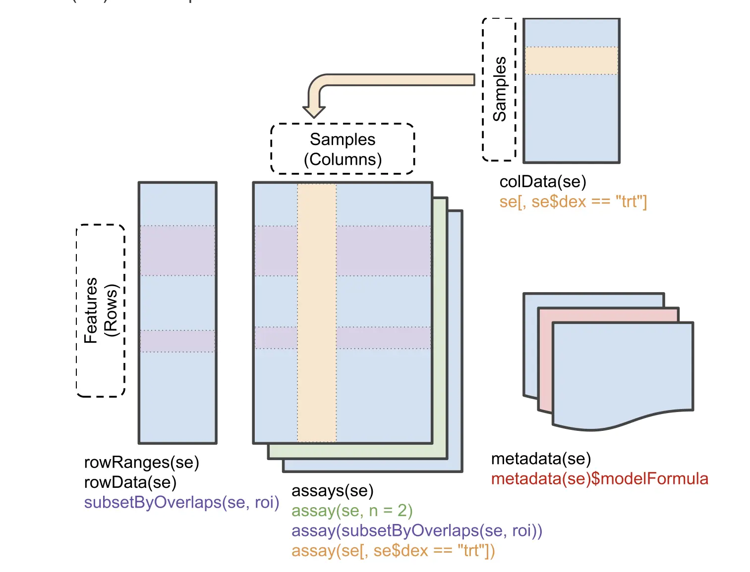
Let’s create an example object here.
## Assays (our matrices)
cnt <- matrix(sample(x = 0:10, size = 9), nrow = 3)
rownames(cnt) <- paste0("gene_", 1:3)
colnames(cnt) <- paste0("sample_", 1:3)
cntNorm <- sweep(cnt, 2, colSums(cnt), "/")*5

## Row information
rd <- DataFrame(chr = as.character(seqnames(gr)),
                chrStart = start(gr),
                chrEnd = end(gr))

## Column information
cd <- DataFrame(condition = c("control", "treatmentA", "treatmentB"))

## Create SE object
se <- SummarizedExperiment(assays = list(counts = cnt, normCounts = cntNorm),
                           rowData = rd, colData = cd)
se
class: SummarizedExperiment
dim: 3 3
metadata(0):
assays(2): counts normCounts
rownames(3): gene_1 gene_2 gene_3
rowData names(3): chr chrStart chrEnd
colnames(3): sample_1 sample_2 sample_3
colData names(1): conditionassays(se)$counts sample_1 sample_2 sample_3
gene_1 2 8 1
gene_2 3 10 6
gene_3 9 0 4rowData(se)DataFrame with 3 rows and 3 columns
chr chrStart chrEnd
<character> <integer> <integer>
gene_1 chr1 30000000 30000040
gene_2 chr2 30000200 30000250
gene_3 chr2 40000800 40000900colData(se)DataFrame with 3 rows and 1 column
condition
<character>
sample_1 control
sample_2 treatmentA
sample_3 treatmentB3 Downloading the data
NoteSetting up and downloading the data
Let’s download the bam files we will be using in this tutorial from Pelle, the HPC from UPPMAX. Make sure you do this in the same working directory you are using. Open a terminal and navigate to your working directory (this is important) and follow these instructions:
## Download the bam files. Replace 'username' with your actual username
mkdir data
rsync username@pelle.uppmax.uu.se:'/proj/uppmax2026-1-197/ChIP/dataMapped/*_chr19.ucsc.fixed.bam*' data/
4 Quality Control (QC)
Let’s begin by doing some QC on the mapped reads. We will be using the QuasR package to do this.
## Create the sample sheet needed by QuasR
## ... See ?qAlign for more details
bamFiles <- file.path(getwd(),
                      list.files("data", pattern = ".bam$", full.names = TRUE))
meta <- data.frame(FileName = bamFiles,
                   SampleName = limma::strsplit2(basename(bamFiles), "_chr19")[, 1])
write.table(meta, file = "data/sampleSheet.txt", quote = FALSE, sep = "\t",
            row.names = FALSE, append = FALSE)

## Create proj object on aligned bam files
## ... you can set the number of cores here according to what works on you machine
cl <- makeCluster(cpus)
proj <- qAlign(sampleFile = "data/sampleSheet.txt",
               genome = "BSgenome.Mmusculus.UCSC.mm39",
               paired = "no",
               clObj = cl,
               checkOnly = TRUE)

## QC plots
dir.create("figures")
qQCReport(input = proj,  pdfFilename = "figures/mappingQC.pdf", clObj=cl)
Examine the generated pdf file and the plots it contains. We like to see high mapping rates typically close to 95% and no big differences in duplicate levels between the samples. Note that here you will see 100% since the bam files have already been filtered for only reads mapping to chr19.
Let’s examine the distribution of the mapping quality scores of the reads in sample ChIPseq_ESC_CTCF_IP_wt_rep1.
## get the mapping quality scores of the reads
bamFile <- "data/ChIPseq_ESC_CTCF_IP_wt_rep1_chr19.ucsc.fixed.bam"
scannedBam <- scanBam(bamFile,
                      param = ScanBamParam(what = c("qname", "mapq")))


## prepare to plot
df <- data.frame(readName = scannedBam[[1]]$qname,
                 mappingScore = scannedBam[[1]]$mapq)

## plot the mapping scores distribution
ggplot(df) +
  geom_histogram(aes(x = mappingScore), bins = 50) +
  theme_bw()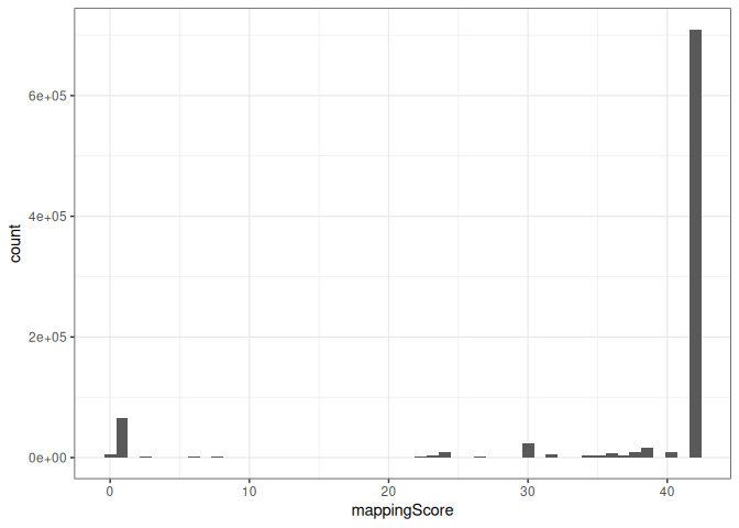
We observe that for this aligner, a mapping score of 42 (which is the maximum here) reflects uniquely aligned reads. We also see that most reads have high mapping scores which is informative for when we want to set cutoffs for minimum mapping quality as we continue with our analyses. Setting a minimum mapping score of 30 when counting for example, we won’t lose that many reads. We can also focus on uniquely mapping reads by setting that minimum to 42.
4.1 GC Bias
An important plot we often look at in ChIP-seq data is the GC-bias trends the samples have. Do they have very different ones and what are the consequences of that?
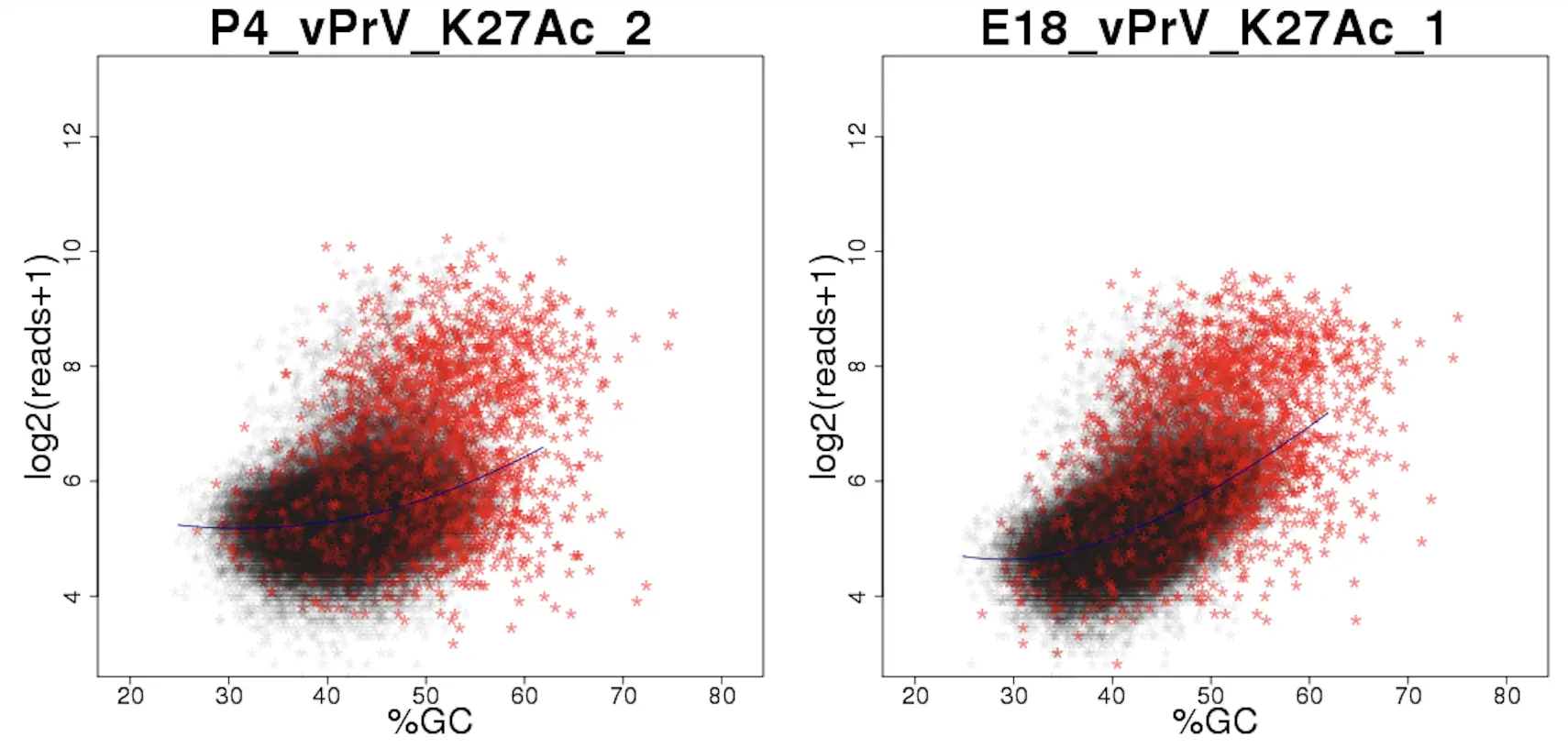
Figure 2 shows very different relationships with GC per condition. The difference is really on the background tiles in black, and this need to be corrected before quantitatively comparing the two samples. Otherwise the difference we see will be driven or explained largely by this difference in GC trend.
Let’s make these plots on the data we have.
## BSgenome
BSgenome <- BSgenome.Mmusculus.UCSC.mm39

## Tile the genome (on chr19 in our case) into 500 bp regions (the tile size
## ... can be set to 1000 or 5000 bp for the histone marks)
tiles <- tileGenome(seqlengths = seqlengths(BSgenome)["chr19"],
                    tilewidth = 500,
                    cut.last.tile.in.chrom = TRUE)
tiles
GRanges object with 122841 ranges and 0 metadata columns:
seqnames ranges strand
<Rle> <IRanges> <Rle>
[1] chr19 1-500 *
[2] chr19 501-1000 *
[3] chr19 1001-1500 *
[4] chr19 1501-2000 *
[5] chr19 2001-2500 *
... ... ... ...
[122837] chr19 61418001-61418500 *
[122838] chr19 61418501-61419000 *
[122839] chr19 61419001-61419500 *
[122840] chr19 61419501-61420000 *
[122841] chr19 61420001-61420004 *
-------
seqinfo: 1 sequence from an unspecified genomeNext, we will make use of the BSgenome object to extract the reference genome sequences and calculate the GC content of each tile.
## Extract the reference genome sequences
tileSeq <- getSeq(BSgenome, tiles)

## Calculate G+C and CpG obs/expected
fMono <- oligonucleotideFrequency(tileSeq, width = 1L, as.prob = TRUE)
fDi <- oligonucleotideFrequency(tileSeq, width = 2L, as.prob = TRUE)
fracGC <- fMono[, "G"] + fMono[, "C"]
oeCpG <- (fDi[, "CG"] + 0.01) / (fMono[, "G"] * fMono[, "C"] + 0.01)

## Add the information to the tiles object
tiles$fracGC <- fracGC
tiles$oeCpG <- oeCpG

## Mark tiles with overlap with CpG islands
## ... if you cloned the repo, you can read it in from the assets folder. Otherwise
## ... you will need to download it from here:
## ... http://hgdownload.cse.ucsc.edu/goldenPath/mm39/database/cpgIslandExt.txt.gz
## ... UCSC bed files are 0-base coordinates so we will have to add +1 to the start position.
cpgFile <- "assets/cpgIslandExt.txt"
cpg <- read.delim(cpgFile, header = FALSE)
cpgGr <- GRanges(
    seqnames = cpg[[2]],
    ranges = IRanges(
        start = cpg[[3]] + 1,
        end = cpg[[4]]
    )
)

ov <- findOverlaps(query = tiles, subject = cpgGr, minoverlap = 5)
cpgTiles <- unique(queryHits(ov))
tiles$overlappingCpG <- ifelse(test = 1:length(tiles) %in% cpgTiles,
                               yes = TRUE, no = FALSE)

head(tiles)
GRanges object with 6 ranges and 3 metadata columns:
seqnames ranges strand | fracGC oeCpG overlappingCpG
<Rle> <IRanges> <Rle> | <numeric> <numeric> <logical>
[1] chr19 1-500 * | 0 1 FALSE
[2] chr19 501-1000 * | 0 1 FALSE
[3] chr19 1001-1500 * | 0 1 FALSE
[4] chr19 1501-2000 * | 0 1 FALSE
[5] chr19 2001-2500 * | 0 1 FALSE
[6] chr19 2501-3000 * | 0 1 FALSE
-------
seqinfo: 1 sequence from an unspecified genome
TipExercise
Examine the different objects above and get more familiar with what they show. You can use the help pages of the used functions with ?functionName to inspect that the functions does, expects and gives back.
We can now proceed to counting the reads on the tiles we have produced. This will take a few seconds.
## Quantify reads
cntTiles <- qCount(proj = proj, query = tiles, mapqMin = 42, clObj = cl)
head(cntTiles)
width ChIPseq_ESC_CTCF_input_BPTFko_rep1 ChIPseq_ESC_CTCF_input_BPTFko_rep2
1 500 0 0
2 500 0 0
3 500 0 0
4 500 0 0
5 500 0 0
6 500 0 0
ChIPseq_ESC_CTCF_input_BPTFko_rep3 ChIPseq_ESC_CTCF_input_BPTFko_rep4
1 0 0
2 0 0
3 0 0
4 0 0
5 0 0
6 0 0
ChIPseq_ESC_CTCF_input_wt_rep1 ChIPseq_ESC_CTCF_input_wt_rep2
1 0 0
2 0 0
3 0 0
4 0 0
5 0 0
6 0 0
ChIPseq_ESC_CTCF_input_wt_rep3 ChIPseq_ESC_CTCF_input_wt_rep4
1 0 0
2 0 0
3 0 0
4 0 0
5 0 0
6 0 0
ChIPseq_ESC_CTCF_IP_BPTFko_rep1 ChIPseq_ESC_CTCF_IP_BPTFko_rep2
1 0 0
2 0 0
3 0 0
4 0 0
5 0 0
6 0 0
ChIPseq_ESC_CTCF_IP_BPTFko_rep3 ChIPseq_ESC_CTCF_IP_BPTFko_rep4
1 0 0
2 0 0
3 0 0
4 0 0
5 0 0
6 0 0
ChIPseq_ESC_CTCF_IP_wt_rep1 ChIPseq_ESC_CTCF_IP_wt_rep2
1 0 0
2 0 0
3 0 0
4 0 0
5 0 0
6 0 0
ChIPseq_ESC_CTCF_IP_wt_rep3 ChIPseq_ESC_CTCF_IP_wt_rep4
1 0 0
2 0 0
3 0 0
4 0 0
5 0 0
6 0 0Let’s plot the log2(counts) vs the GC content of the tiles.
## Prepare to plot
## ... We randomly subsample 25,000 tiles for faster plotting and
## ... exclude tiles which have zero counts in all samples
df <- as.data.frame(cbind(cntTiles, mcols(tiles)))
zeroCounts <- rowSums(cntTiles[, -1]) == 0
sum(zeroCounts) / nrow(df)
[1] 0.09631963df <- df[!zeroCounts, ]
set.seed(123)
i <- sample(x = 1:nrow(df), size = 25000, replace = FALSE)
df <- df[i, ]
df <- df %>%
as_tibble() %>%
pivot_longer(cols = starts_with("ChIPseq_"), names_to = "sample", values_to = "rawCount")
## Plot
ggplot(df, aes(x = fracGC, y = log2(rawCount+1))) +
geom_point(size = 0.3) +
theme_bw() +
facet_wrap(~sample)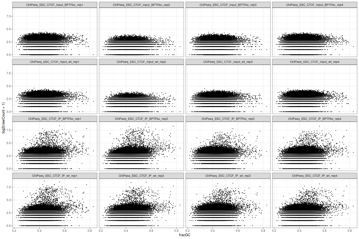
Compare the input samples to those where the TF was pulled down. What do you notice?
In this data set we notice a few things. Firstly, there is no relationship between count and GC content. It looks to be flat. Secondly, the samples have the same relationship between read count and GC content. If we had considerable differences in GC trends between samples we wish to quantitatively compare we would have had to normalize them accordingly before comparing them or doing differential analyses, as the differences in counts could be largely driven by differences in GC trends. We will explore more how to correct for this in the advanced ChIP-seq tutorial.
Notice that the cloud above the background represents tiles with signal, where the TF is bound. Another thing to look out for is how similar the signal or enrichment is for these samples. Was there one replicate which had a very poor signal for instance?
TipExercise
Re-do the plots above, coloring by oeCpG and overlappingCpG. Depending on the ChIP, the signal can sometimes overlap with CpG islands. Do you see this here?
4.2 Global correlation
Another quick QC step already at the tile level, is to look at how the samples group together. Ideally, we want to see replicates of the same condition grouping together, unless there are other reasons they shouldn’t. For example if the signals differ a lot between samples and that drives the correlation, if the biological source of variation between conditions is smaller than the technical source of variation, or if there are no biological differences between conditions.
First, we need to normalize for difference in library size between samples. Let’s do this by calculating counts per million. Briefly, for each sample, each tile’s count is divided by the total number of reads in that sample and then multiplied by 1 million to get counts per million (CPM).
## log2(CPM+1)
cpm <- sweep(x = cntTiles[, -1],
             MARGIN = 2,
             STATS = colSums(cntTiles[, -1]),
             FUN = "/")*1e6
log2cpm <- log2(cpm + 1)

## Shorten the sample names
colnames(log2cpm) <- gsub("ChIPseq_ESC_CTCF_", "", colnames(log2cpm))

## Pearson correlation
cor <- cor(log2cpm)

## Plot correlation heatmap
Heatmap(cor, name = "Pears Corr")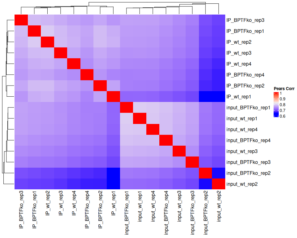
We can notice a separation between input and IP samples. Within the IP samples we don’t see obvious groupings based on condition (wt or BPTFko). This may be due to most tiles being background noise and this dominating the correlation. We will see later if this improves when looking at the peak count matrix.
4.3 Enrichment over the input sample
Let’s next use the tile count matrix to calculate enrichment values for the IP samples. We will first calculate normalized counts, correcting for library size differences between samples.
## Normalized count matrix
cnt <- cntTiles[, -1]
medianLib <- median(colSums(cnt))
cntNorm <- sweep(cnt, MARGIN = 2, STATS = colSums(cnt), FUN = "/") * medianLib
log2cntNorm <- log2(cntNorm + 8)
TipExercise
Compare the library sizes before and after correction. You can use colSums to sum the reads per sample.
Let’s calculate the enrichment values over the input for all samples. The enrichment will be calculated as \(enr=log_2\frac{(normCountIP+8)}{(normCountInput+8)}\).
## Samples
samples <- apply(limma::strsplit2(colnames(cnt), "_")[, 5:6],
                 MARGIN = 1,
                 FUN = function(x){paste(x, collapse = "_")})
spl <- split(colnames(cnt), samples)
spl
$BPTFko_rep1
[1] "ChIPseq_ESC_CTCF_input_BPTFko_rep1" "ChIPseq_ESC_CTCF_IP_BPTFko_rep1"
$BPTFko_rep2
[1] "ChIPseq_ESC_CTCF_input_BPTFko_rep2" "ChIPseq_ESC_CTCF_IP_BPTFko_rep2"
$BPTFko_rep3
[1] "ChIPseq_ESC_CTCF_input_BPTFko_rep3" "ChIPseq_ESC_CTCF_IP_BPTFko_rep3"
$BPTFko_rep4
[1] "ChIPseq_ESC_CTCF_input_BPTFko_rep4" "ChIPseq_ESC_CTCF_IP_BPTFko_rep4"
$wt_rep1
[1] "ChIPseq_ESC_CTCF_input_wt_rep1" "ChIPseq_ESC_CTCF_IP_wt_rep1"
$wt_rep2
[1] "ChIPseq_ESC_CTCF_input_wt_rep2" "ChIPseq_ESC_CTCF_IP_wt_rep2"
$wt_rep3
[1] "ChIPseq_ESC_CTCF_input_wt_rep3" "ChIPseq_ESC_CTCF_IP_wt_rep3"
$wt_rep4
[1] "ChIPseq_ESC_CTCF_input_wt_rep4" "ChIPseq_ESC_CTCF_IP_wt_rep4" ## Calculate enrichment of input for all IP samples
enr <- do.call(cbind, lapply(spl, function(samples){
ip <- samples[grep("_IP_", samples)]
input <- samples[grep("_input_", samples)]
log2cntNorm[, ip] - log2cntNorm[, input]
}))
head(enr) BPTFko_rep1 BPTFko_rep2 BPTFko_rep3 BPTFko_rep4 wt_rep1 wt_rep2 wt_rep3
1 0 0 0 0 0 0 0
2 0 0 0 0 0 0 0
3 0 0 0 0 0 0 0
4 0 0 0 0 0 0 0
5 0 0 0 0 0 0 0
6 0 0 0 0 0 0 0
wt_rep4
1 0
2 0
3 0
4 0
5 0
6 0We can now look at the distribution of these enrichment values. Let’s have a look at sample wt_rep1.
## Prepare to plot
df <- as.data.frame(enr) %>%
  pivot_longer(cols = everything(), names_to = "sample", values_to = "enr") %>%
  dplyr::filter(sample == "wt_rep1")

## Plot
ggplot(df) +
  geom_histogram(aes(x = enr), bins = 60) +
  theme_bw()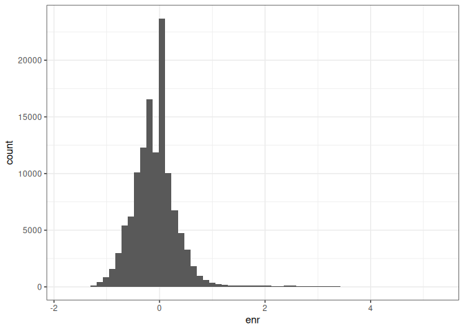
The normal looking distribution shows the background, and we can set a cutoff at around 2 to select for tiles which we consider enriched for the TF. Let’s do that and see where these tiles fall in the count vs GC plot.
## Label enriched tiles for wt_rep1
enrTiles <- enr[, "wt_rep1"] > 2

## Prepare to plot
df <- as.data.frame(cbind(cntTiles, mcols(tiles)))
df$enrTiles <- enrTiles
df$enr <- enr[, "wt_rep1"]
zeroCounts <- rowSums(cntTiles[, -1]) == 0
sum(zeroCounts) / nrow(df)
[1] 0.09631963df <- df[!zeroCounts, ]
set.seed(123)
i <- sample(x = 1:nrow(df), size = 25000, replace = FALSE)
df <- df[i, ]
df <- df %>%
as_tibble() %>%
pivot_longer(cols = starts_with("ChIPseq_"), names_to = "sample", values_to = "rawCount") %>%
dplyr::filter(sample == "ChIPseq_ESC_CTCF_IP_wt_rep1")
## Plot
p1 <- ggplot(df, aes(x = fracGC, y = log2(rawCount+1))) +
geom_point(aes(color = enr), size = 0.3) +
scale_color_viridis_c() +
theme_bw()
p2 <- ggplot(df, aes(x = fracGC, y = log2(rawCount+1))) +
geom_point(aes(color = enrTiles), size = 0.3) +
theme_bw()
p1 + p2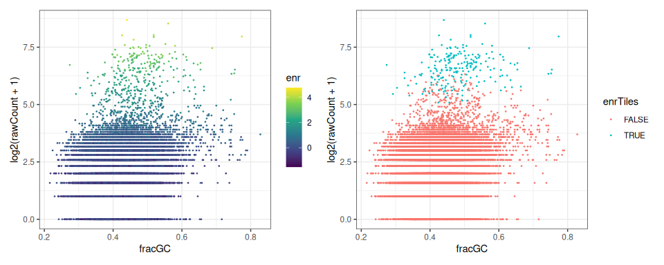
5 Estimating the fragment size
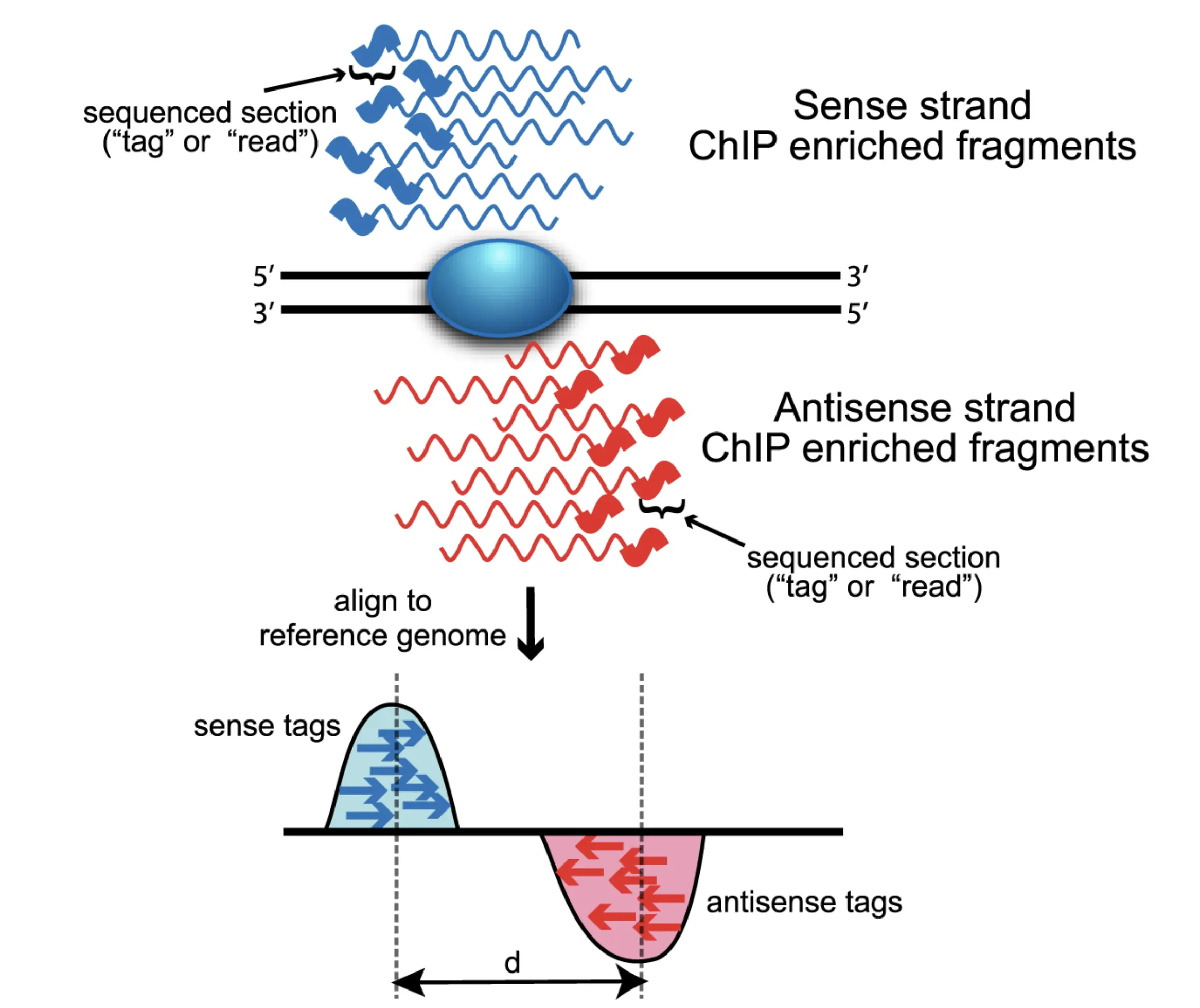
ChIP-seq enriches the DNA fragments containing the bound TF, and so the reads start at the beginning of the fragment. This does not reflect where the TF was sitting, likely somewhere in the middle of the fragment. To have the reads reflect the position of the TF, which is our signal of interest, the reads need to be shifted by a size which approximately translates to half the fragment size. Figure 3 from Wilbanks and Facciotti (2010) illustrates this. Our samples contain single end (SE) reads, some coming from the negative and some the positive strand. We can use this to estimate the original fragment size by shifting the reads from the forward strand and calculating the cross-correlation between the shifted forward positions and the original reverse positions.
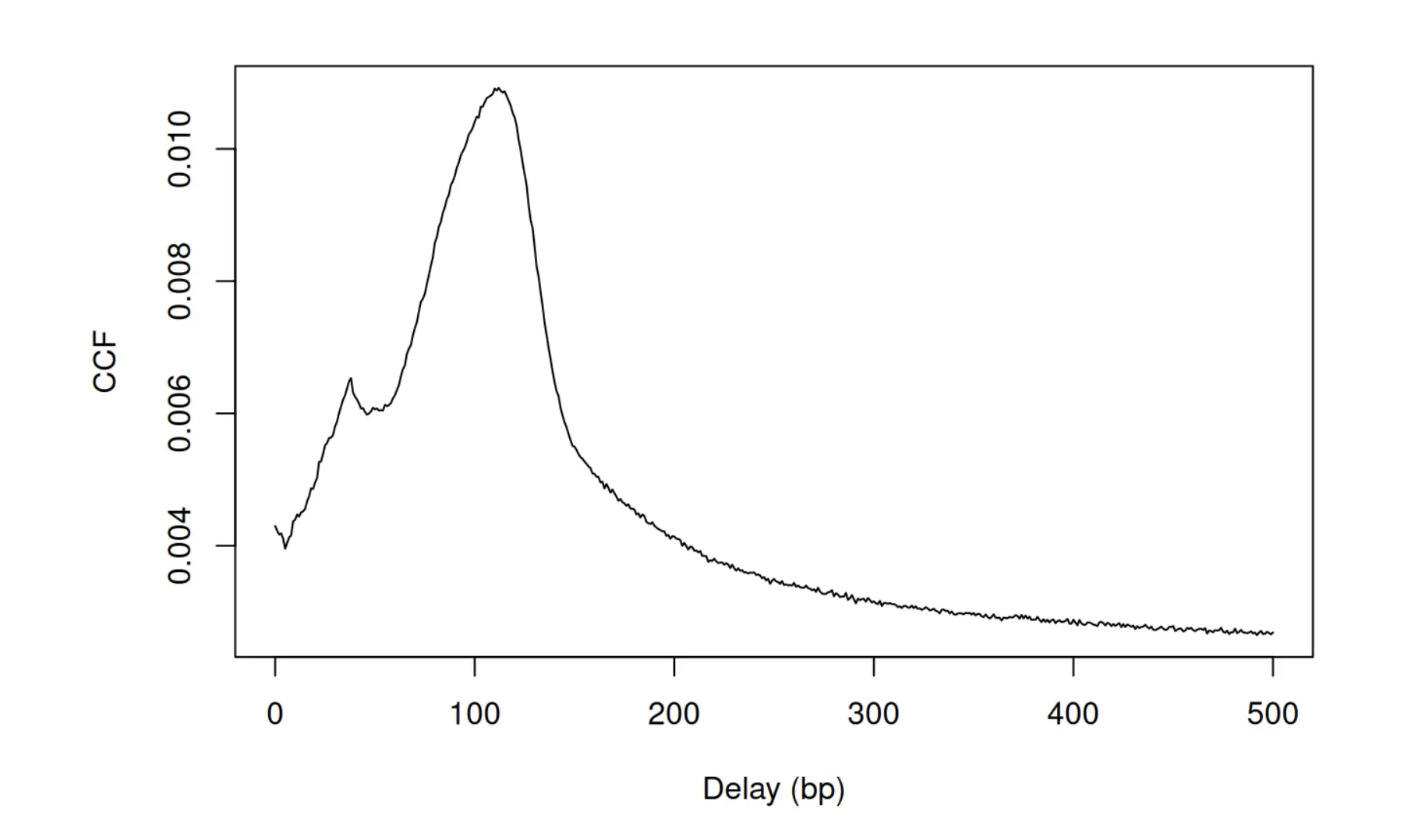
Let’s take one example sample and estimate the average fragment size. Note that this needs to be a non-input sample.
## Estimate the fragment size
bamFile <- "data/ChIPseq_ESC_CTCF_IP_wt_rep1_chr19.ucsc.fixed.bam"
param <- readParam(minq=30)
maxDelay <- 500
ccf <- correlateReads(bamFile, maxDelay, param=param)

## prepare to plot
df <- data.frame(ccf = ccf,
                 shiftInBasePairs = 0:maxDelay)

## plot
ggplot(df, aes(x = shiftInBasePairs, y = ccf)) +
  geom_line() +
  theme_bw()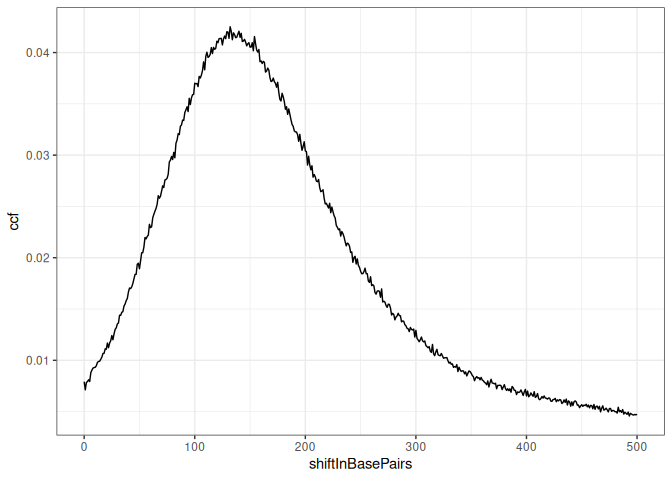
We can get the value of the shift at the maximum peak, which will correspond to the estimated fragment size.
maximizeCcf(ccf)[1] 132
TipExercise
Choose another sample and estimate the average fragment size. How does it compare to ChIPseq_ESC_CTCF_IP_wt_rep1? By how much should the reads be shifted on average to get the TF binding location, and in what direction?
6 Peak calling
Shifting the forward and reverse reads by half the fragment size will be important during peak calling. We will be using MACS3 for peak calling. MACS stands for Model-based Analysis of ChIP-Seq. The main function we will be using there is callpeak. Note that we have chipped for TFs and so need to call narrow peaks representing the TF binding site. When chipping histone marks such as H3K27-acetylation, we expect broader peaks and there we would need to add the --broad argument when doing peak calling. We will also make use of our input samples when peak calling. This will be useful, especially since we have experiments on cell lines (ESCs), so that we can avoid problematic and repetitive parts of the genome which may appear as false peaks otherwise. This should be less of a problem in in-vivo data, but having inputs is always a benefit to be able to avoid false peaks especially when comparing different samples.
The peak caller will by default filter duplicates by keeping one duplicate read both in the IP and its input sample. It will also estimate the average fragment size and shift the reads accordingly before doing peak calling. Generally speaking, peak calling is done by using a sliding window and comparing the counts in that to a background sliding window to see if there are more counts than expected. For more details on how peak calling is done in MACS3 see this section in the manual. You can also have a look at all the parameters the aligner offers by using macs3 -h.
Let’s do peak calling on the ChIPseq_ESC_CTCF_IP_wt_rep1 sample. Note that this step needs to done on Pelle (the HPC from UPPMAX). If you are unable to access the compute server, you may skip this step for now. We will be reading in the called peaks later. Note that we need to specify the effective genome size value which is the size of the mappable genome. Because of the repetitive features on the chromosomes, the actual mappable genome size will be smaller than the original size, about 90% or 70% of the genome size. You can find more information and suggested values here. Since we are only looking at chr19 in these bam files, we will set it to the size of that chromosome (even though in reality the mappable size will be smaller), but this should be modified accordingly when working with the full genome.
## MACS3 functions
macs3=/proj/uppmax2026-1-197/ChIP/software/pixiEnvs/macs3/macs3-v3.0.4/.pixi/envs/default/bin/macs3
$macs3 --help
$macs3 callpeak --help

## Specify parameters
bamIP=/proj/uppmax2026-1-197/ChIP/dataMapped/ChIPseq_ESC_CTCF_IP_wt_rep1_chr19.ucsc.fixed.bam
bamInput=/proj/uppmax2026-1-197/ChIP/dataMapped/ChIPseq_ESC_CTCF_input_wt_rep1_chr19.ucsc.fixed.bam
genomeSize=61420004
sampleName=ChIPseq_ESC_CTCF_wt_rep1

## Peak calling on the sample
## ... note that one can relax the q parameter a bit and allow for more false
## ... peaks as they don't have a critical global impact when we produce the
## ... count matrix.
$macs3 callpeak -t $bamIP -c $bamInput -f BAM -g $genomeSize -q 0.01 \
    -n $sampleName --outdir ChIPpeaks
This command has been run for the rest of the samples. We will now download the peaks bed files and then read them into R.
TipExercise
Check the contents of the ChIPpeaks folder. You can have a look at the individual files using less yourFileName, and exit this with q (short for quit).
NoteDownloading the peak files
Make sure you do this in the same working directory you are using. Open a terminal and navigate to your working directory (this is important) and follow these instructions:
## Download the peak files. Replace 'username' with your Pelle username.
mkdir peaks
rsync username@pelle.uppmax.uu.se:'/proj/uppmax2026-1-197/ChIP/peaks/*_peaks.narrowPeak' peaks/
6.1 Peak overlap
Let’s examine how well our peaks overlap, particularly the replicates.
## Read in peaks
peakFiles <- list.files("peaks", full.names = TRUE)
names(peakFiles) <- gsub("_chr19_peaks.narrowPeak", "", basename(peakFiles))
peaksL <- lapply(peakFiles, function(bedFile){import(bedFile)})
peaksL$ChIPseq_ESC_CTCF_IP_BPTFko_rep1
GRanges object with 1163 ranges and 6 metadata columns:
seqnames ranges strand | name score
<Rle> <IRanges> <Rle> | <character> <numeric>
[1] chr19 3059550-3059819 * | ChIPseq_ESC_CTCF_IP_.. 257
[2] chr19 3258311-3258615 * | ChIPseq_ESC_CTCF_IP_.. 727
[3] chr19 3273770-3273994 * | ChIPseq_ESC_CTCF_IP_.. 95
[4] chr19 3278304-3278564 * | ChIPseq_ESC_CTCF_IP_.. 133
[5] chr19 3332885-3333111 * | ChIPseq_ESC_CTCF_IP_.. 175
... ... ... ... . ... ...
[1159] chr19 61086260-61086499 * | ChIPseq_ESC_CTCF_IP_.. 199
[1160] chr19 61098642-61098950 * | ChIPseq_ESC_CTCF_IP_.. 283
[1161] chr19 61187855-61188121 * | ChIPseq_ESC_CTCF_IP_.. 367
[1162] chr19 61254191-61254377 * | ChIPseq_ESC_CTCF_IP_.. 99
[1163] chr19 61254891-61255161 * | ChIPseq_ESC_CTCF_IP_.. 486
signalValue pValue qValue peak
<numeric> <numeric> <numeric> <integer>
[1] 8.62671 28.5884 25.75100 129
[2] 16.38670 76.4159 72.72480 151
[3] 5.57114 12.0869 9.56585 90
[4] 6.80638 15.9299 13.32920 124
[5] 8.18234 20.2028 17.51420 112
... ... ... ... ...
[1159] 6.29569 22.7298 19.98930 107
[1160] 10.31520 31.2332 28.34810 122
[1161] 8.76285 39.7359 36.70950 198
[1162] 6.00291 12.5126 9.98652 68
[1163] 15.23010 51.9089 48.68680 132
-------
seqinfo: 1 sequence from an unspecified genome; no seqlengths## Generate all sample pair combinations we wish to look for peak Overlap.
samplePairs <- combn(names(peaksL), 2, simplify = FALSE)
names(samplePairs) <- samplePairs
## Count overlaps in all sample pairs with min overlap set to 5 bases
ovL <- lapply(samplePairs, function(samples){
sum(countOverlaps(peaksL[[samples[1]]], peaksL[[samples[2]]], minoverlap = 5))
})
## Create symmetric samples matrix showing the number of pairwise overlaps
samples <- names(peaksL)
ovMat <- matrix(
0,
nrow = length(samples),
ncol = length(samples),
dimnames = list(samples, samples)
)
for (i in seq_along(ovL)) {
x <- names(ovL)[i]
x <- sub('^c\\(\\"', '', x)
x <- sub('\\"\\)$', '', x)
x <- strsplit(x, '\\", \\"')[[1]]
s1 <- x[1]
s2 <- x[2]
ovMat[s1, s2] <- ovL[[i]]
ovMat[s2, s1] <- ovL[[i]]
}
diag(ovMat) <- NA
## Calculate fraction of peaks overlapping
all(names(peaksL) == colnames(ovMat))[1] TRUEcolnames(ovMat) <- gsub("ChIPseq_ESC_CTCF_", "", colnames(ovMat))
rownames(ovMat) <- gsub("ChIPseq_ESC_CTCF_", "", rownames(ovMat))
fracOvMat <- sweep(x = ovMat, MARGIN = 1, STATS = lengths(peaksL), FUN = "/")
## Plot
H1 <- Heatmap(ovMat, name = "numberOverlaps",
column_title = "Number of Overlapping Peaks")
H2 <- Heatmap(fracOvMat, name = "fracOverlaps",
column_title = "Fraction of Overlapping Peaks")
H1 + H2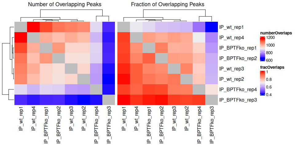
Here we also don’t see an obvious grouping of samples by condition (wt vs BPTFko). This could be due to reasons related to overall lower signal and lots of background noise.
Note that we are looking at pairwise overlaps. Below we make use of the plotOverlaps function from the extraChIPs package to look at how well the peaks in each sample agree with the rest. Under the hood this is creating a union set of peaks and checking if each sample overlaps this set, so the numbers don’t reflect the true number of peaks we have here.
plotOverlaps(GRangesList(peaksL), type = "upset")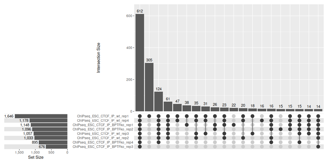
It’s only at bar number 7 where we see 35 peaks shared only in the wt replicates. Otherwise most peaks seem shared, although the wt_rep1 sample has a lot of unique peaks.
7 Count reads on peaks
Let’s create a common set of peaks that we can use to create a count matrix across all samples so we can have a more global and quantitative overview of how well the samples agree.
## Define common set of peaks as the union
peaks <- reduce(unlist(GRangesList(peaksL)))
head(peaks)
GRanges object with 6 ranges and 0 metadata columns:
seqnames ranges strand
<Rle> <IRanges> <Rle>
[1] chr19 3059528-3059881 *
[2] chr19 3254545-3255056 *
[3] chr19 3255261-3255425 *
[4] chr19 3258301-3258877 *
[5] chr19 3273692-3274050 *
[6] chr19 3278242-3278564 *
-------
seqinfo: 1 sequence from an unspecified genome; no seqlengthslength(peaks)[1] 1752
TipExercise
Plot the histogram of the peak widths for the unified set of peaks. Do these widths make sense for a TF? What do you think this would look like for a histone mark like H3K27Ac?
Let’s count the reads on the peaks. Now that we have made use of the input samples during peak calling we will ignore them for the time being and on focus on the counts of the IP samples.
## Count reads across peaks (shifting by 1/2 the fragment length).
## ... Looking at the output of fragment size estimates (d) in MACS3 in the .xls
## ... files, the median across all samples is 150, so we will shift by 75 in
## ... the 3' direction.
cntPeaks <- qCount(proj = proj, query = peaks, mapqMin = 42, clObj = cl,
                   shift = 75)

## Only keep IP samples
cntPeaks <- cntPeaks[, grepl("_IP_", colnames(cntPeaks))]
head(cntPeaks)
ChIPseq_ESC_CTCF_IP_BPTFko_rep1 ChIPseq_ESC_CTCF_IP_BPTFko_rep2
1 0 0
2 7 14
3 0 0
4 42 47
5 1 1
6 0 0
ChIPseq_ESC_CTCF_IP_BPTFko_rep3 ChIPseq_ESC_CTCF_IP_BPTFko_rep4
1 0 0
2 3 9
3 0 1
4 23 27
5 0 0
6 0 0
ChIPseq_ESC_CTCF_IP_wt_rep1 ChIPseq_ESC_CTCF_IP_wt_rep2
1 0 0
2 45 39
3 5 5
4 54 42
5 3 3
6 0 0
ChIPseq_ESC_CTCF_IP_wt_rep3 ChIPseq_ESC_CTCF_IP_wt_rep4
1 0 0
2 26 37
3 0 2
4 34 28
5 4 1
6 0 0Let’s now create a SummarizedExperiment object for the peaks count matrix. We will also add additional information on the peaks like GC content, position etc. This way everything we need is on one object.
## Calculate G+C and CpG obs/expected
peaksSeq <- getSeq(BSgenome, peaks)
fMono <- oligonucleotideFrequency(peaksSeq, width = 1L, as.prob = TRUE)
fDi <- oligonucleotideFrequency(peaksSeq, width = 2L, as.prob = TRUE)
fracGC <- fMono[, "G"] + fMono[, "C"]
oeCpG <- (fDi[, "CG"] + 0.01) / (fMono[, "G"] * fMono[, "C"] + 0.01)

## Add the information to the peaks
peaks$fracGC <- fracGC
peaks$oeCpG <- oeCpG

## Mark peaks with overlap with CpG islands
ov <- findOverlaps(query = peaks, subject = cpgGr, minoverlap = 5)
cpgPeaks <- unique(queryHits(ov))
peaks$overlappingCpG <- ifelse(test = 1:length(peaks) %in% cpgPeaks,
                               yes = TRUE, no = FALSE)

## Annotate peaks:
## ... overlapping gene (overlapping any transcript)
## ... distal: at least 1 kb away from any transcription start site (TSS) and
## ... not overlapping a transcript
## ... overlapping promoters (1kb around tss)
## ... other
peaks$type <- rep("other", length(peaks))
txdb <- TxDb.Mmusculus.UCSC.mm39.knownGene
txs <- transcripts(txdb)
ov <- findOverlaps(peaks, txs)
peaks$type[unique(queryHits(ov))] <- "gene"
tss <- resize(txs, width = 1)
dist <- distanceToNearest(x = peaks, subject = tss)
dist <- elementMetadata(dist)$distance
peaks$type[dist >= 1000 & peaks$type != "gene"] <- "distal"
promoters <- tss + 1000
ov <- findOverlaps(peaks, promoters)
peaks$type[unique(queryHits(ov))] <- "promoter"

## View peaks GRanges
head(peaks)
GRanges object with 6 ranges and 4 metadata columns:
seqnames ranges strand | fracGC oeCpG overlappingCpG
<Rle> <IRanges> <Rle> | <numeric> <numeric> <logical>
[1] chr19 3059528-3059881 * | 0.403955 0.531515 FALSE
[2] chr19 3254545-3255056 * | 0.472656 0.277827 FALSE
[3] chr19 3255261-3255425 * | 0.533333 0.127982 FALSE
[4] chr19 3258301-3258877 * | 0.377816 0.563893 FALSE
[5] chr19 3273692-3274050 * | 0.473538 0.534199 FALSE
[6] chr19 3278242-3278564 * | 0.482972 0.556218 FALSE
type
<character>
[1] distal
[2] promoter
[3] promoter
[4] distal
[5] distal
[6] distal
-------
seqinfo: 1 sequence from an unspecified genome; no seqlengths## View peak types
table(peaks$type)
  distal     gene promoter
     373      938      441
## Prepare for SummarizedExperiment object
rd <- as.data.frame(peaks) %>%
rename(chr = seqnames, chrStart = start, chrEnd = end,
peakWidth = width, chrStrand = strand)
rd <- DataFrame(rd)
cd <- DataFrame(sampleName = apply(X = limma::strsplit2(colnames(cntPeaks), "_")[, 5:6],
MARGIN = 1,
FUN = function(x){paste(x, collapse = "_")}),
genotype = limma::strsplit2(colnames(cntPeaks), "_")[, 5])
## Make SE object
se <- SummarizedExperiment(assays = list(counts = cntPeaks),
rowData = rd,
colData = cd)
rownames(se) <- paste0("peak_", 1:nrow(se))
colnames(se) <- cd$sampleName
seclass: SummarizedExperiment
dim: 1752 8
metadata(0):
assays(1): counts
rownames(1752): peak_1 peak_2 ... peak_1751 peak_1752
rowData names(9): chr chrStart ... overlappingCpG type
colnames(8): BPTFko_rep1 BPTFko_rep2 ... wt_rep3 wt_rep4
colData names(2): sampleName genotyperowData(se)DataFrame with 1752 rows and 9 columns
chr chrStart chrEnd peakWidth chrStrand fracGC oeCpG
<factor> <integer> <integer> <integer> <factor> <numeric> <numeric>
peak_1 chr19 3059528 3059881 354 * 0.403955 0.531515
peak_2 chr19 3254545 3255056 512 * 0.472656 0.277827
peak_3 chr19 3255261 3255425 165 * 0.533333 0.127982
peak_4 chr19 3258301 3258877 577 * 0.377816 0.563893
peak_5 chr19 3273692 3274050 359 * 0.473538 0.534199
... ... ... ... ... ... ... ...
peak_1748 chr19 61119450 61119815 366 * 0.469945 0.533657
peak_1749 chr19 61187832 61188199 368 * 0.546196 0.660310
peak_1750 chr19 61212424 61212574 151 * 0.377483 0.223537
peak_1751 chr19 61253769 61254469 701 * 0.446505 0.239460
peak_1752 chr19 61254868 61255170 303 * 0.574257 0.869759
overlappingCpG type
<logical> <character>
peak_1 FALSE distal
peak_2 FALSE promoter
peak_3 FALSE promoter
peak_4 FALSE distal
peak_5 FALSE distal
... ... ...
peak_1748 FALSE gene
peak_1749 FALSE promoter
peak_1750 FALSE gene
peak_1751 FALSE promoter
peak_1752 TRUE promotercolData(se)DataFrame with 8 rows and 2 columns
sampleName genotype
<character> <character>
BPTFko_rep1 BPTFko_rep1 BPTFko
BPTFko_rep2 BPTFko_rep2 BPTFko
BPTFko_rep3 BPTFko_rep3 BPTFko
BPTFko_rep4 BPTFko_rep4 BPTFko
wt_rep1 wt_rep1 wt
wt_rep2 wt_rep2 wt
wt_rep3 wt_rep3 wt
wt_rep4 wt_rep4 wt
TipExercise
Subset the se object, keeping peaks which have a GC fraction greater than 0.5 and keeping the samples which are wt only. Make sure to store it into a new variable for example seSub. Access the counts, rowData and colData in this new object. Are they also subsetted? The point here is to illustrate how these objects can be used.
8 Scatter plots
We will next make scatter plots comparing all samples against each other and color by density. This is also an important QC plot to see if there are global trends that differ a lot between the samples and if there is a need to correct for them, assuming we do not expect genome-wide differences between samples. This can be for instance driven by differences in the count vs GC content trends.
## Create a CPM matrix (correting for library size differences)
cpm <- sweep(x = assays(se)$counts, MARGIN = 2,
             STATS = colSums(assays(se)$counts), FUN = "/")*1e6
log2cpm <- log2(cpm + 1)

## Add to the SE object
assays(se)$cpm <- cpm
assays(se)$log2cpm <- log2cpm
se
class: SummarizedExperiment
dim: 1752 8
metadata(0):
assays(3): counts cpm log2cpm
rownames(1752): peak_1 peak_2 ... peak_1751 peak_1752
rowData names(9): chr chrStart ... overlappingCpG type
colnames(8): BPTFko_rep1 BPTFko_rep2 ... wt_rep3 wt_rep4
colData names(2): sampleName genotype## Pairs plot
jet.colors <- colorRampPalette(c("#00007F", "blue", "#007FFF", "cyan",
"#7FFF7F", "yellow", "#FF7F00", "red", "#7F0000"))
pairs(assays(se)$log2cpm, panel = function(...){
smoothScatter(..., nrpoints = 0, colramp = jet.colors, add=TRUE);
abline(a=0,b=1,col="white")}, main = "log2(CPM+1")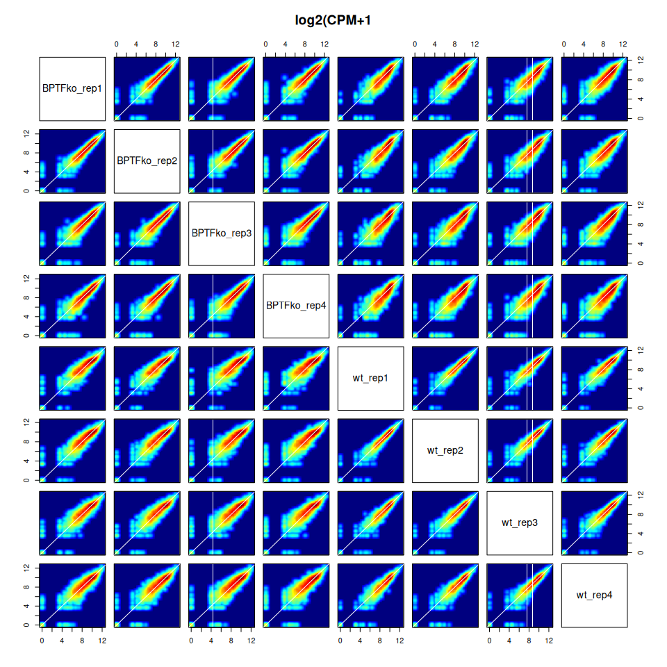
We can notice that for all comparisons, most data points fall on the diagonal (white line) indicating no global shifts or non-linearities we need to worry about. The density is reflected in the colors, the more red the more dense that part of the plot is. Notice also that within a condition, for example within wt, the scatter plots look more narrow (globally more similar) to each other, and that this becomes a little bit wider when you compare to the samples from the other contiditon. Take wt_rep4 for instance and compare it against the other samples above.
9 Global groupings
Let’s revisit the correlation heatmap. Earlier we did this on the tiles and did not see clear groupings. Can we see better groupings in the peaks count matrix? Focusing on the peaks should improve our signal, since the tiles will contain a lot of noisy background counts, especially with TF ChIP-seq, where we expect most tiles not to have the TF bound.
## Correlation heatmap
cor <- cor(assays(se)$log2cpm)
Heatmap(cor, name = "Pears Corr")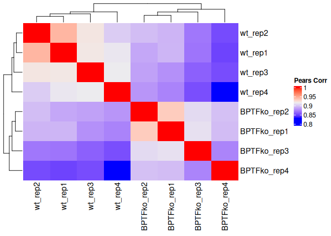
We can nicely see the samples grouping by condition.
Let’s also do a PCA (Principal Component Analysis) on the log2(CPM) count matrix. We would like to know how the samples group in the high dimensional peak space but there are too many peaks (dimensions) to be able to get a sense of this visually (we can at most have a plot of 2 or 3 dimensions or axes). The PCA will map our samples onto a new set of coordinates or principal components (PCs), ordered from highest to lowest by the variance explained in the data.
## PCA
pca <- prcomp(x = t(assays(se)$log2cpm), center = TRUE, scale. = FALSE)
s <- summary(pca)
s
Importance of components:
PC1 PC2 PC3 PC4 PC5 PC6 PC7
Standard deviation 17.3522 12.2342 10.4536 9.9774 8.69491 8.28178 6.93668
Proportion of Variance 0.3534 0.1757 0.1283 0.1168 0.08874 0.08051 0.05648
Cumulative Proportion 0.3534 0.5291 0.6574 0.7743 0.86301 0.94352 1.00000
PC8
Standard deviation 1.948e-14
Proportion of Variance 0.000e+00
Cumulative Proportion 1.000e+00Notice that we have 8 PCs (because we have 8 samples) and that the “Proportion of Variance” sums to 100% across all PCs.
## Prepare to plot
pc1var <- round(s$importance["Proportion of Variance", "PC1"]*100, digits = 2)
pc2var <- round(s$importance["Proportion of Variance", "PC2"]*100, digits = 2)
pc3var <- round(s$importance["Proportion of Variance", "PC3"]*100, digits = 2)
df <- cbind(as.data.frame(pca$x), colData(se))

## Plot
ggplot(df, aes(x = PC1, y = PC2)) +
  geom_point(aes(color = genotype)) +
  labs(title = "PCA", x = paste0("PC1 (", pc1var, "%)"), y = paste0("PC2 (", pc2var, "%)")) +
  coord_fixed(ratio = pc2var/pc1var) +
  theme_bw()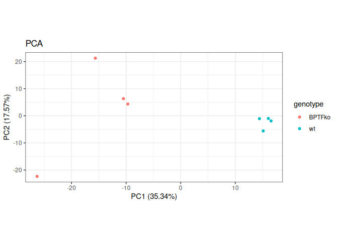
PC1 which captures around 35% of the variance is separating the wt from the BPTFko condition. This is informative and indicates that our biological signal of interest (the difference between the two conditions) is nicely explaining a big source of variance. Notice also that in this PC1 and PC2 space, the wt samples seem to group together more tightly whereas the BPTFko samples are a little more scattered indicating more variation between the replicates there, captured in PC2.
10 Profile plots
The called peaks should reflect the binding sites of the CTCF TF. Let’s take the peaks, center them and look at the overall reads distribution, comparing the BPTFko to the wt. We will use QuasR to create these profile plots.
## Center peaks
centeredPeaks <- resize(peaks, width = 1, fix = "center")
centeredPeaks
GRanges object with 1752 ranges and 4 metadata columns:
seqnames ranges strand | fracGC oeCpG overlappingCpG
<Rle> <IRanges> <Rle> | <numeric> <numeric> <logical>
[1] chr19 3059704 * | 0.403955 0.531515 FALSE
[2] chr19 3254800 * | 0.472656 0.277827 FALSE
[3] chr19 3255343 * | 0.533333 0.127982 FALSE
[4] chr19 3258589 * | 0.377816 0.563893 FALSE
[5] chr19 3273871 * | 0.473538 0.534199 FALSE
... ... ... ... . ... ... ...
[1748] chr19 61119632 * | 0.469945 0.533657 FALSE
[1749] chr19 61188015 * | 0.546196 0.660310 FALSE
[1750] chr19 61212499 * | 0.377483 0.223537 FALSE
[1751] chr19 61254119 * | 0.446505 0.239460 FALSE
[1752] chr19 61255019 * | 0.574257 0.869759 TRUE
type
<character>
[1] distal
[2] promoter
[3] promoter
[4] distal
[5] distal
... ...
[1748] gene
[1749] promoter
[1750] gene
[1751] promoter
[1752] promoter
-------
seqinfo: 1 sequence from an unspecified genome; no seqlengths## Create profile
profile <- qProfile(proj, query = centeredPeaks, upstream = 1000,
downstream = 1000, orientation = "any",
shift = 75, clObj = cl)
names(profile) [1] "coverage" "ChIPseq_ESC_CTCF_input_BPTFko_rep1"
[3] "ChIPseq_ESC_CTCF_input_BPTFko_rep2" "ChIPseq_ESC_CTCF_input_BPTFko_rep3"
[5] "ChIPseq_ESC_CTCF_input_BPTFko_rep4" "ChIPseq_ESC_CTCF_input_wt_rep1"
[7] "ChIPseq_ESC_CTCF_input_wt_rep2" "ChIPseq_ESC_CTCF_input_wt_rep3"
[9] "ChIPseq_ESC_CTCF_input_wt_rep4" "ChIPseq_ESC_CTCF_IP_BPTFko_rep1"
[11] "ChIPseq_ESC_CTCF_IP_BPTFko_rep2" "ChIPseq_ESC_CTCF_IP_BPTFko_rep3"
[13] "ChIPseq_ESC_CTCF_IP_BPTFko_rep4" "ChIPseq_ESC_CTCF_IP_wt_rep1"
[15] "ChIPseq_ESC_CTCF_IP_wt_rep2" "ChIPseq_ESC_CTCF_IP_wt_rep3"
[17] "ChIPseq_ESC_CTCF_IP_wt_rep4" We can see the number of summed reads at each position relative to the center of the peaks.
profile$ChIPseq_ESC_CTCF_IP_BPTFko_rep1[, 1:10]-1000 -999 -998 -997 -996 -995 -994 -993 -992 -991
49 44 48 40 58 38 54 51 34 43 Next we will normalize the counts for library size difference between the samples. Note that in our case we are summing the reads over the same set of peaks across the samples. However, one can also make these plots on groups of regions by naming the regions by the group they should belong to. Reads belonging to the same group are summed up. In this case one will also want to normalize for differences in the number of regions per group which is captured in the coverage matrix of the returned list.
## Calculate scaling factors to normalize for the library size difference
libSizes <- alignmentStats(proj)[, "mapped"]
sf <- libSizes / median(libSizes)
sf
ChIPseq_ESC_CTCF_input_BPTFko_rep1:genome
0.9904982
ChIPseq_ESC_CTCF_input_BPTFko_rep2:genome
0.5778143
ChIPseq_ESC_CTCF_input_BPTFko_rep3:genome
0.7529092
ChIPseq_ESC_CTCF_input_BPTFko_rep4:genome
0.9060492
ChIPseq_ESC_CTCF_input_wt_rep1:genome
0.9735194
ChIPseq_ESC_CTCF_input_wt_rep2:genome
0.5452840
ChIPseq_ESC_CTCF_input_wt_rep3:genome
0.8193324
ChIPseq_ESC_CTCF_input_wt_rep4:genome
0.9592341
ChIPseq_ESC_CTCF_IP_BPTFko_rep1:genome
1.1202356
ChIPseq_ESC_CTCF_IP_BPTFko_rep2:genome
1.0996593
ChIPseq_ESC_CTCF_IP_BPTFko_rep3:genome
1.1154957
ChIPseq_ESC_CTCF_IP_BPTFko_rep4:genome
1.0789751
ChIPseq_ESC_CTCF_IP_wt_rep1:genome
1.0095018
ChIPseq_ESC_CTCF_IP_wt_rep2:genome
1.1499849
ChIPseq_ESC_CTCF_IP_wt_rep3:genome
1.1693313
ChIPseq_ESC_CTCF_IP_wt_rep4:genome
1.0621019 ## Aggregate into one matrix
profileMat <- do.call(rbind, profile[2:length(profile)])
rownames(profileMat) <- names(profile)[2:length(profile)]
profileMat[, 1:10] -1000 -999 -998 -997 -996 -995 -994 -993
ChIPseq_ESC_CTCF_input_BPTFko_rep1 36 37 37 24 25 37 24 29
ChIPseq_ESC_CTCF_input_BPTFko_rep2 27 12 24 14 10 20 15 16
ChIPseq_ESC_CTCF_input_BPTFko_rep3 13 32 30 20 21 20 27 14
ChIPseq_ESC_CTCF_input_BPTFko_rep4 14 25 26 29 35 19 19 29
ChIPseq_ESC_CTCF_input_wt_rep1 24 34 21 25 30 30 34 24
ChIPseq_ESC_CTCF_input_wt_rep2 19 18 21 16 13 14 18 19
ChIPseq_ESC_CTCF_input_wt_rep3 27 17 24 25 15 28 22 28
ChIPseq_ESC_CTCF_input_wt_rep4 29 29 27 31 31 22 19 18
ChIPseq_ESC_CTCF_IP_BPTFko_rep1 49 44 48 40 58 38 54 51
ChIPseq_ESC_CTCF_IP_BPTFko_rep2 45 58 48 44 58 54 55 50
ChIPseq_ESC_CTCF_IP_BPTFko_rep3 42 35 44 54 44 46 52 25
ChIPseq_ESC_CTCF_IP_BPTFko_rep4 53 40 40 41 44 35 50 39
ChIPseq_ESC_CTCF_IP_wt_rep1 48 52 62 50 46 37 54 49
ChIPseq_ESC_CTCF_IP_wt_rep2 50 57 57 45 46 49 44 39
ChIPseq_ESC_CTCF_IP_wt_rep3 41 51 49 48 43 60 50 35
ChIPseq_ESC_CTCF_IP_wt_rep4 20 35 49 41 41 47 41 56
-992 -991
ChIPseq_ESC_CTCF_input_BPTFko_rep1 29 27
ChIPseq_ESC_CTCF_input_BPTFko_rep2 14 25
ChIPseq_ESC_CTCF_input_BPTFko_rep3 22 28
ChIPseq_ESC_CTCF_input_BPTFko_rep4 30 16
ChIPseq_ESC_CTCF_input_wt_rep1 21 35
ChIPseq_ESC_CTCF_input_wt_rep2 8 18
ChIPseq_ESC_CTCF_input_wt_rep3 28 21
ChIPseq_ESC_CTCF_input_wt_rep4 24 28
ChIPseq_ESC_CTCF_IP_BPTFko_rep1 34 43
ChIPseq_ESC_CTCF_IP_BPTFko_rep2 53 37
ChIPseq_ESC_CTCF_IP_BPTFko_rep3 52 38
ChIPseq_ESC_CTCF_IP_BPTFko_rep4 36 49
ChIPseq_ESC_CTCF_IP_wt_rep1 41 53
ChIPseq_ESC_CTCF_IP_wt_rep2 49 40
ChIPseq_ESC_CTCF_IP_wt_rep3 50 37
ChIPseq_ESC_CTCF_IP_wt_rep4 45 40## Normalize reads for library size differences
profileMat <- sweep(x = profileMat, MARGIN = 1, STATS = sf, FUN = "/")
## Prepare to plot
df <- as.data.frame(profileMat) %>%
rownames_to_column("sampleName") %>%
mutate(sampleName = gsub("ChIPseq_ESC_CTCF_", "", sampleName),
condition = sub("_rep[0-9]+$", "", sampleName)) %>%
pivot_longer(cols = -c(sampleName, condition),
names_to = "position",
values_to = "normCount") %>%
mutate(position = as.numeric(position))
## Plot
ggplot(df, aes(x = position, y = normCount)) +
geom_line(aes(group = sampleName, color = condition)) +
theme_bw() 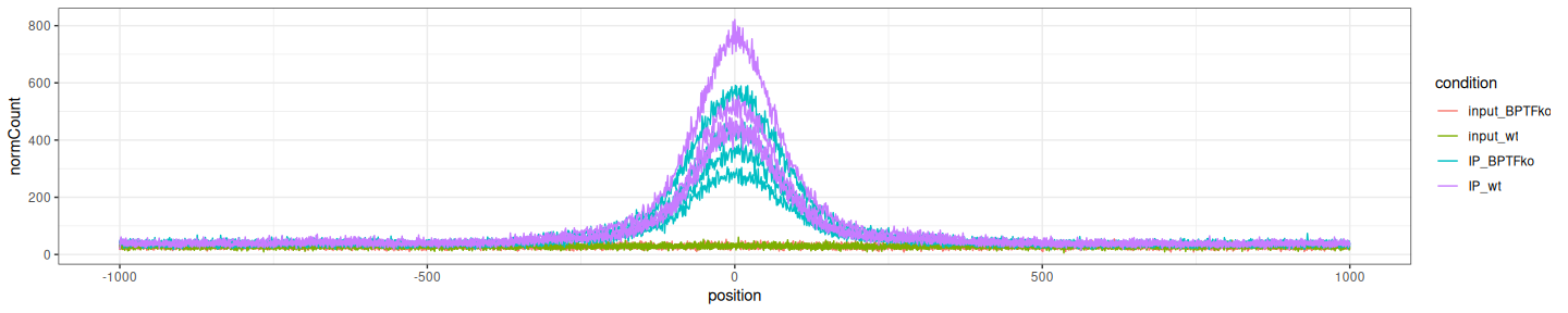
We can see flat lines for the input samples, and on average, a global reduction in CTCF binding in the BPTFko samples compared to the wt. Remember that position 0 reflects the midpoint of the peaks. Here we made these profile plots using all peaks as regions, but you can do this on any regions of interest. For example if you have accessibility data on the same samples, one could ask, is there a reduction in CTCF binding in regions which lose accessibility or regions which stay constantly accessible?
TipExercise
Use the qProfile and centeredPeaks object on an IP sample of choice and do the counting without shifting the reads. Make the profile plot. Do you see a bimodal distribution reflecting the fragment length? You can select one sample by substituting the proj object (e.g. projSub <- proj[16]). You can skip the library size correction step since we are looking at one sample. Make sure that the rows in centeredPeaks have the same name so that the reads are summed up, instead of counted per peak.
11 Heatmaps on peaks
Another way to visualize this is via a heatmap. Here we need to make sure to provide the qProfile function with a GRanges where each peak has a unique name, so that the counts are not summed up over the peaks.
## Profile plot counting on each peak
names(centeredPeaks) <- paste0("peak_", 1:length(centeredPeaks))
profile <- qProfile(proj, query = centeredPeaks, upstream = 1000,
                    downstream = 1000, orientation = "any",
                    shift = 75, clObj = cl)
head(profile$ChIPseq_ESC_CTCF_IP_BPTFko_rep1[, 1:10])
-1000 -999 -998 -997 -996 -995 -994 -993 -992 -991
peak_1 0 0 0 0 0 0 0 0 0 0
peak_2 0 0 0 0 0 0 0 0 0 0
peak_3 0 0 0 0 0 0 0 0 0 0
peak_4 0 0 0 0 0 0 0 0 0 0
peak_5 0 0 0 0 0 0 0 0 0 0
peak_6 0 0 0 0 0 0 0 0 0 0Let’s normalize these raw count matrices for library size differences again, and this time sum up the reads per condition (sum the replicates) to have an aggregate view.
## Normalize for library size diffs
normProfile <- lapply(2:length(profile), function(i){
  profile[[i]] / sf[i-1]
})
names(normProfile) <- names(sf)

## Sum counts (matrices) by condition
spl <- split(names(normProfile),
             paste(limma::strsplit2(names(normProfile), "_")[, 4],
                   limma::strsplit2(names(normProfile), "_")[, 5],
                   sep = "_"))
summedNormProfile <- lapply(spl, function(samples) {
    Reduce(`+`, normProfile[samples])
})

## Prepare for heatmaps on the peaks with the biggest absolute log2 fold-change
## ... between BPTFko and wt
avrPeakLogFC <- rowMeans(assays(se)$log2cpm[, grep("BPTFko", colnames(se))]) -
  rowMeans(assays(se)$log2cpm[, grep("wt", colnames(se))])
topVar <- abs(avrPeakLogFC) > 1.5
matWt <- summedNormProfile$IP_wt[topVar, ]
matBptfko <- summedNormProfile$IP_BPTFko[topVar, ]
matDiff <- matBptfko - matWt

## Heatmaps
peakClust <- hclust(dist(matDiff), method = "ward.D2")
colFunCnt <- colorRamp2(
    c(quantile(rbind(matWt, matBptfko), 0.05), quantile(rbind(matWt, matBptfko), 0.95)),
    c("cornsilk", "firebrick4")
)
colFunDiff <- colorRamp2(
    c(-2, 0, 2),
    c("steelblue", "cornsilk", "coral")
)
colsToLabel <- c("-800", "-400", "0", "400", "800")
columnLabels <- ifelse(
    colnames(matDiff) %in% colsToLabel,
    colnames(matDiff),
    ""
)

H1 <- Heatmap(matWt, cluster_columns = FALSE, show_row_names = FALSE,
              cluster_rows = peakClust, use_raster = TRUE, name = "normWtCount",
              column_title = "CTCF Binding Around Peaks in Wt",
              col = colFunCnt, column_labels = columnLabels,
              column_names_side = "top")
H2 <- Heatmap(matBptfko, cluster_columns = FALSE, show_row_names = FALSE,
              cluster_rows = peakClust, use_raster = TRUE, name = "normBPTFkoCount",
              column_title = "CTCF Binding Around Peaks in BPTFko",
              col = colFunCnt, column_labels = columnLabels,
              column_names_side = "top")
H3 <- Heatmap(matDiff, cluster_columns = FALSE, show_row_names = FALSE,
              cluster_rows = peakClust, use_raster = TRUE, name = "BPTFko-wt",
              column_title = "CTCF Binding Around Peaks in (BPTFko - Wt)",
              col = colFunDiff, column_labels = columnLabels,
              column_names_side = "top")
H1 + H2 + H3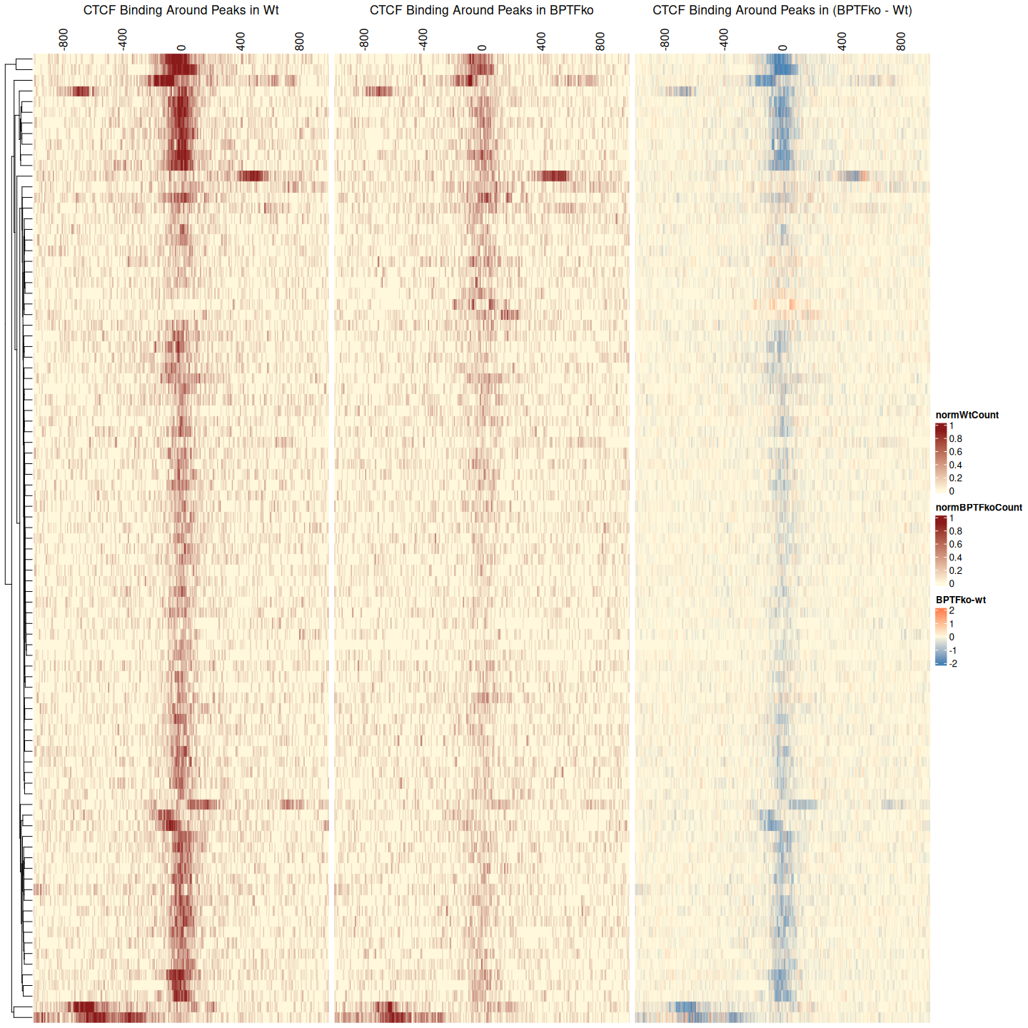
We can see clear losses of CTCF binding in the top variable peaks.
12 Differential binding
For the differential binding let’s first plot the log2 fold change between BPTFko and wt vs the average exrpession across all samples. We want to see most points centered on the y=0 line and no non-linearities. This plot is often called an MA plot. Notice that there is more variability for low expression and that this variability decreases with a higher average count.
## Calculate log2FC(BPTFko cpm / wt cpm)
cpm <- assays(se)$cpm
cpm <- cpm + 1
cpmWt <- rowMeans(cpm[, grep("wt", colnames(cpm))])
cpmBPTFko <- rowMeans(cpm[, grep("BPTFko", colnames(cpm))])
log2FC <- log2((cpmBPTFko)/(cpmWt))
log2avrCPM <- log2(rowMeans(cpm))

## Plot
df <- data.frame(log2FC = log2FC, log2avrCPM = log2avrCPM)
ggplot(df, aes(x = log2avrCPM, y = log2FC)) +
  geom_point() +
  geom_hline(yintercept = 0, linetype = "dashed", color = "steelblue") +
  theme_bw()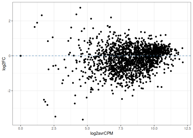
## Design matrix
condition <- as.factor(colData(se)$genotype)
design <- model.matrix(~0+condition)
colnames(design) <- levels(condition)
design
BPTFko wt
1 1 0
2 1 0
3 1 0
4 1 0
5 0 1
6 0 1
7 0 1
8 0 1
attr(,"assign")
[1] 1 1
attr(,"contrasts")
attr(,"contrasts")$condition
[1] "contr.treatment"## Prepare DGE object for edgeR
dge <- DGEList(counts = assays(se)$counts, group = condition, genes = rowData(se))
## Library sizes
dge$samples| group | lib.size | norm.factors | |
|---|---|---|---|
| BPTFko_rep1 | BPTFko | 92033 | 1 |
| BPTFko_rep2 | BPTFko | 116690 | 1 |
| BPTFko_rep3 | BPTFko | 62599 | 1 |
| BPTFko_rep4 | BPTFko | 74447 | 1 |
| wt_rep1 | wt | 128073 | 1 |
| wt_rep2 | wt | 103168 | 1 |
| wt_rep3 | wt | 90592 | 1 |
| wt_rep4 | wt | 82793 | 1 |
## Correct for library size diffs
dge <- normLibSizes(dge)
dge$samples| group | lib.size | norm.factors | |
|---|---|---|---|
| BPTFko_rep1 | BPTFko | 92033 | 0.9935899 |
| BPTFko_rep2 | BPTFko | 116690 | 0.9786221 |
| BPTFko_rep3 | BPTFko | 62599 | 0.9851050 |
| BPTFko_rep4 | BPTFko | 74447 | 0.9702059 |
| wt_rep1 | wt | 128073 | 1.0408106 |
| wt_rep2 | wt | 103168 | 1.0194295 |
| wt_rep3 | wt | 90592 | 1.0057661 |
| wt_rep4 | wt | 82793 | 1.0083365 |
## Filter out peaks with low counts
## ... This will keep peaks which have CPM >= CPM.cutoff in MinSampleSize samples
## ... where CPM.cutoff = min.count / median(lib.size) * 1e6
keep <- filterByExpr(dge)
dge <- dge[keep, ]

## Fraction kept peaks with enough counts
sum(keep) / length(peaks)
[1] 0.8464612## Normalize for lib sizes again (since the total lib size changes after excluding some peaks)
dge <- normLibSizes(dge)
dge$samples| group | lib.size | norm.factors | |
|---|---|---|---|
| BPTFko_rep1 | BPTFko | 92033 | 0.9951907 |
| BPTFko_rep2 | BPTFko | 116690 | 0.9881437 |
| BPTFko_rep3 | BPTFko | 62599 | 0.9883282 |
| BPTFko_rep4 | BPTFko | 74447 | 0.9751885 |
| wt_rep1 | wt | 128073 | 1.0251907 |
| wt_rep2 | wt | 103168 | 1.0109642 |
| wt_rep3 | wt | 90592 | 1.0085630 |
| wt_rep4 | wt | 82793 | 1.0093467 |
## Estimate disperion
dge <- estimateDisp(y=dge, design=design)
## Fit model
fit <- glmQLFit(dge, design)## Contrast: BPTFko vs wt
contrast <- makeContrasts(BPTFko-wt, levels=design)
diffTest <- glmQLFTest(fit, contrast=contrast)
diffTable <- as.data.frame(topTags(diffTest, n = nrow(dge)))
head(diffTable)| chr | chrStart | chrEnd | peakWidth | chrStrand | fracGC | oeCpG | overlappingCpG | type | logFC | logCPM | F | PValue | FDR | |
|---|---|---|---|---|---|---|---|---|---|---|---|---|---|---|
| peak_1719 | chr19 | 60149323 | 60149741 | 419 | * | 0.4319809 | 0.7709960 | FALSE | gene | -1.732190 | 10.591162 | 177.79381 | 0 | 0e+00 |
| peak_528 | chr19 | 12465428 | 12465861 | 434 | * | 0.5460829 | 0.3108814 | FALSE | gene | -1.706001 | 10.311449 | 155.81798 | 0 | 0e+00 |
| peak_1269 | chr19 | 44618072 | 44618650 | 579 | * | 0.4283247 | 0.4035638 | FALSE | gene | 1.213981 | 10.864000 | 114.47167 | 0 | 0e+00 |
| peak_1432 | chr19 | 47000984 | 47001298 | 315 | * | 0.4825397 | 0.5250812 | FALSE | gene | -1.847189 | 9.243506 | 93.46690 | 0 | 0e+00 |
| peak_676 | chr19 | 22992876 | 22993242 | 367 | * | 0.4686649 | 0.2823977 | FALSE | gene | -1.398932 | 9.766961 | 80.42600 | 0 | 1e-07 |
| peak_499 | chr19 | 11142635 | 11142955 | 321 | * | 0.5482866 | 0.4844686 | FALSE | promoter | -1.775814 | 9.135681 | 79.31345 | 0 | 1e-07 |
ggplot(diffTable, aes(x = logCPM, y = logFC)) +
  geom_point(aes(color = FDR <= 0.05)) +
  geom_hline(yintercept = 0, linetype = "dashed") +
  theme_bw()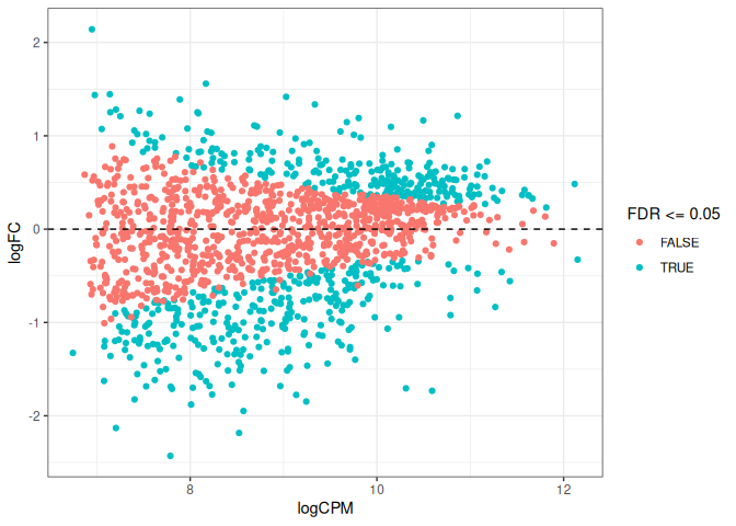
ggplot(diffTable, aes(x = logCPM, y = logFC)) +
  geom_point(aes(color = FDR <= 0.05 & abs(logFC) >= 1.5)) +
  geom_hline(yintercept = 0, linetype = "dashed") +
  theme_bw()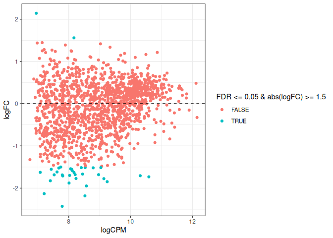
Let’s take these top peaks with differential binding and look at the peak by sample heatmap. How well do the replicates agree, and are some of these peaks clearly different or less so.
## log2cpm of top diff peaks
diffPeaks <- rownames(diffTable)[diffTable$FDR <= 0.05 & abs(diffTable$logFC) >= 1.5]
log2cpm <- assays(se)$log2cpm[diffPeaks, ]

## log2FC with respect to mean across samples
log2cpmFC <- sweep(x = log2cpm, MARGIN = 1, STATS = rowMeans(log2cpm), FUN = "-")
log2cpmFC <- as.matrix(log2cpmFC)

## Plot
Heatmap(log2cpmFC, name = "log2FC w.r.t. mean")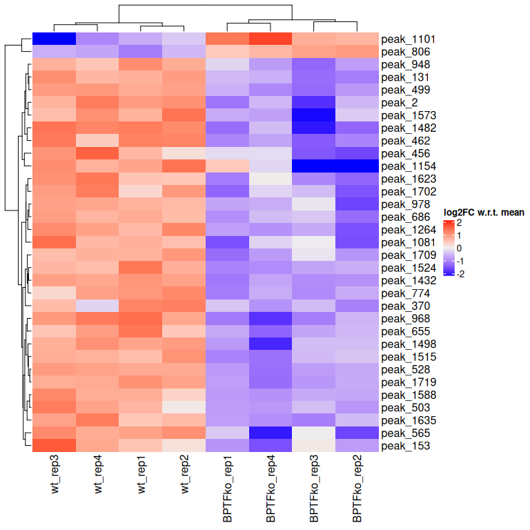
We can appreciate a strong agreement between replicates within a condition.
13 Visualize peaks on genome tracks
Let’s choose a peak that is showing strong differential binding between BPTFko and wt, and visualize the count tracks on the reference genome. We will choose peak_462, which according to the heatmap above shows loss of CTCF binding in the BPTFko condition.
First, we will need to produce BigWig files for each sample. BigWig files are a file format used to visualize continuous data in the genome browser. We will use the qExportWig function from QuasR to produce these files, shifting the reads by 75 bases in the 3’ direction and setting the binsize to 100. Reads are scaled by the total number of reads to correct for library size differences between samples. See the help page of the qExportWig function for more details.
## Create BigWig files (this can take a few seconds)
dir.create("bigwigs")
bwFiles <- file.path("bigwigs",
                     paste0(basename(alignments(proj)$genome$SampleName), ".bw"))
bwFiles <- gsub("ChIPseq_ESC_CTCF_", "", bwFiles)
qExportWig(proj, file = bwFiles, binsize = 100, shift = 75,
           createBigWig = TRUE, clObj = cl)
## Read in BigWigs
names(bwFiles) <- gsub(".bw", "", basename(bwFiles))
bwGrL <- lapply(bwFiles, function(file){
import(file)
})
head(bwGrL$IP_BPTFko_rep1)GRanges object with 6 ranges and 1 metadata column:
seqnames ranges strand | score
<Rle> <IRanges> <Rle> | <numeric>
[1] chr1 1-100 * | 0
[2] chr1 101-200 * | 0
[3] chr1 201-300 * | 0
[4] chr1 301-400 * | 0
[5] chr1 401-500 * | 0
[6] chr1 501-600 * | 0
-------
seqinfo: 61 sequences from an unspecified genomeSince we have input samples we will include them in our visualization. They are a good check to have that we aren’t looking at a false signal.
## Get peak coordinates and add 8kb upstream and downstream
trackStart <- rowData(se)["peak_462", ]$chrStart - 15000
trackEnd <- rowData(se)["peak_462", ]$chrEnd + 15000

## Set y-axis limit to be the same
ylims <- c(0, max(sapply(bwGrL, function(gr){
  keep <- seqnames(gr) == "chr19" & start(gr) >= trackStart & end(gr) <= trackEnd
  grSub <- gr[keep]
  max(grSub$score)})))

## Prepare sample tracks
cols <- c(
  input_wt = "grey",
  input_BPTFko = "grey",
  IP_wt = "forestgreen",
  IP_BPTFko = "firebrick"
)
tracks <- lapply(names(bwGrL), function(sn){
  cond <- sub("_rep[0-9]$", "", sn)
  DataTrack(range = bwGrL[[sn]],
            name = sn,
            type = "histogram",
            fill = cols[cond],
            just.title = "center")
})

## Prepare genome and gene annotations track
genomeTrack <- GenomeAxisTrack()
txdb <- TxDb.Mmusculus.UCSC.mm39.knownGene
genes <- genes(txdb)
geneTrack <- GeneRegionTrack(genes, genome = "mm39",
                             chromosome = "chr19",
                             name = "Genes",
                             rotation.title = 0)
chrTrack <- IdeogramTrack(genome = "mm39", chromosome = "chr19")

## Prepare peak track
peaksGr <- makeGRangesFromDataFrame(rowData(se))
peaksGr$peakName = names(peaksGr)
peakTrack <- AnnotationTrack(peaksGr, name = "Peaks", rotation.title = 0)

## Plot tracks
plotTracks(c(chrTrack, genomeTrack, tracks, peakTrack),
           chromosome="chr19",
           from = trackStart,
           to = trackEnd,
           ylim = ylims, title.width = 2, cex.title = 0.5, just.title = "center")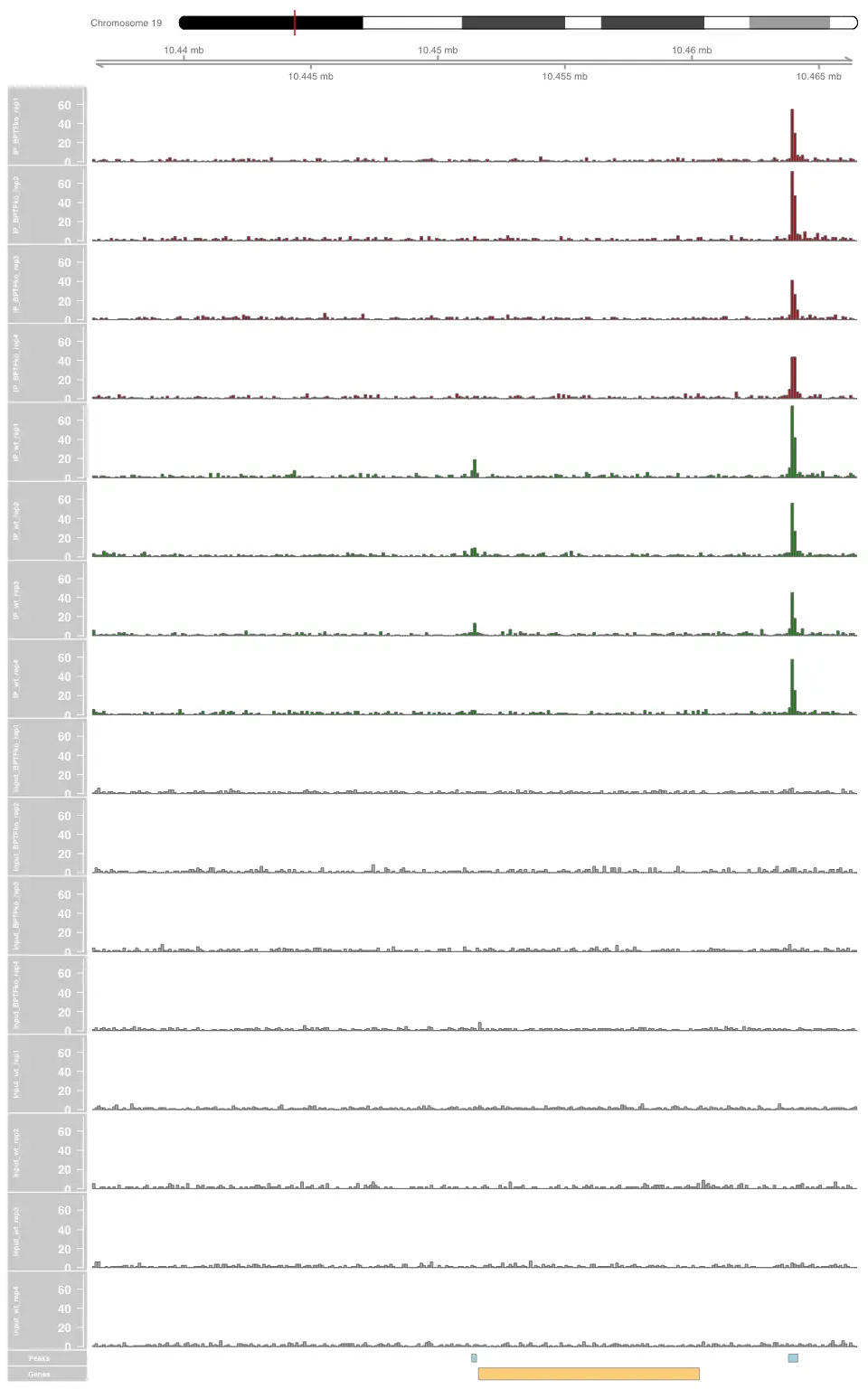
We can appreciate the benefit and importance of having several replicates per condition to detect constant changes in signal, especially smaller changes in signal. This becomes even more important for TFs that are hard to pull down or experiments where we see a lot of background noise. In the figure above we can for example see that for wt_rep4 the CTCF signal for our peak of interest was not as high as the other 3 replicates. When examining and placing importance on individual peaks and interpreting them correctly, having several replicates is necessary to be sure of the effect we are seeing beyond variability between replicates.
TipExercise
Pick another peak(s) and make the same plot. Feel free to alter the range around the peak you wish to see.
14 Session
date()Code Output
[1] "Fri Oct 9 13:39:00 2026"sessionInfo()Code Output
R version 4.6.1 (2026-06-24)
Platform: x86_64-pc-linux-gnu
Running under: Ubuntu 24.04.5 LTS

Matrix products: default
BLAS:   /usr/lib/x86_64-linux-gnu/openblas-pthread/libblas.so.3
LAPACK: /usr/lib/x86_64-linux-gnu/openblas-pthread/libopenblasp-r0.3.26.so;  LAPACK version 3.12.0

locale:
 [1] LC_CTYPE=C.UTF-8       LC_NUMERIC=C           LC_TIME=C.UTF-8
 [4] LC_COLLATE=C.UTF-8     LC_MONETARY=C.UTF-8    LC_MESSAGES=C.UTF-8
 [7] LC_PAPER=C.UTF-8       LC_NAME=C              LC_ADDRESS=C
[10] LC_TELEPHONE=C         LC_MEASUREMENT=C.UTF-8 LC_IDENTIFICATION=C

time zone: UTC
tzcode source: system (glibc)

attached base packages:
 [1] grid      stats4    parallel  stats     graphics  grDevices datasets
 [8] utils     methods   base

other attached packages:
 [1] edgeR_4.10.3
 [2] Gviz_1.56.0
 [3] extraChIPs_1.16.2
 [4] ggside_0.4.1
 [5] BiocParallel_1.46.0
 [6] SimpleUpset_0.1.6
 [7] dplyr_1.2.1
 [8] tibble_3.3.1
 [9] tidyr_1.3.2
[10] circlize_0.4.18
[11] ComplexHeatmap_2.28.0
[12] patchwork_1.3.2
[13] ggplot2_4.0.3
[14] Rsamtools_2.28.0
[15] csaw_1.46.0
[16] SummarizedExperiment_1.42.0
[17] MatrixGenerics_1.24.0
[18] matrixStats_1.5.0
[19] TxDb.Mmusculus.UCSC.mm39.knownGene_3.22.0
[20] GenomicFeatures_1.64.0
[21] AnnotationDbi_1.74.0
[22] Biobase_2.72.0
[23] BSgenome.Mmusculus.UCSC.mm39_1.4.3
[24] BSgenome_1.80.0
[25] rtracklayer_1.72.0
[26] BiocIO_1.22.0
[27] Biostrings_2.80.0
[28] XVector_0.52.0
[29] limma_3.68.5
[30] QuasR_1.52.0
[31] Rbowtie_1.52.0
[32] GenomicRanges_1.64.0
[33] Seqinfo_1.2.0
[34] IRanges_2.46.0
[35] S4Vectors_0.50.2
[36] BiocGenerics_0.58.1
[37] generics_0.1.4

loaded via a namespace (and not attached):
  [1] splines_4.6.1            bitops_1.0-9             filelock_1.0.3
  [4] XML_3.99-0.23            rpart_4.1.27             lifecycle_1.0.5
  [7] httr2_1.2.2              pwalign_1.8.0            doParallel_1.0.17
 [10] lattice_0.22-9           ensembldb_2.36.1         GenomicFiles_1.48.0
 [13] backports_1.5.1          magrittr_2.0.5           Hmisc_5.3-0
 [16] rmarkdown_2.31           yaml_2.3.12              metapod_1.20.0
 [19] otel_0.2.0               DBI_1.3.0                RColorBrewer_1.1-3
 [22] abind_1.4-8              ShortRead_1.70.0         purrr_1.2.2
 [25] AnnotationFilter_1.36.0  biovizBase_1.60.0        RCurl_1.98-1.18
 [28] nnet_7.3-20              VariantAnnotation_1.58.0 rappdirs_0.3.4
 [31] ggrepel_0.9.8            codetools_0.2-20         DelayedArray_0.38.1
 [34] tidyselect_1.2.1         shape_1.4.6.1            UCSC.utils_1.8.0
 [37] farver_2.1.2             BiocFileCache_3.2.0      base64enc_0.1-6
 [40] GenomicAlignments_1.48.0 jsonlite_2.0.0           GetoptLong_1.1.1
 [43] Formula_1.2-6            iterators_1.0.14         foreach_1.5.2
 [46] tools_4.6.1              progress_1.2.3           Rcpp_1.1.1-1.1
 [49] glue_1.8.1               gridExtra_2.3.1          SparseArray_1.12.2
 [52] xfun_0.57                GenomeInfoDb_1.48.0      withr_3.0.2
 [55] BiocManager_1.30.27      fastmap_1.2.0            latticeExtra_0.6-31
 [58] digest_0.6.39            R6_2.6.1                 colorspace_2.1-2
 [61] jpeg_0.1-11              dichromat_2.0-1          biomaRt_2.68.0
 [64] RSQLite_3.53.1           cigarillo_1.2.0          renv_1.2.3
 [67] data.table_1.18.6.1      prettyunits_1.2.0        InteractionSet_1.40.0
 [70] httr_1.4.8               htmlwidgets_1.6.4        S4Arrays_1.12.1
 [73] pkgconfig_2.0.3          gtable_0.3.6             blob_1.3.0
 [76] S7_0.2.2                 hwriter_1.3.2.1          htmltools_0.5.9
 [79] ProtGenerics_1.44.0      clue_0.3-68              scales_1.4.0
 [82] png_0.1-9                knitr_1.51               rstudioapi_0.19.0
 [85] rjson_0.2.23             checkmate_2.3.4          curl_7.1.0
 [88] cachem_1.1.0             GlobalOptions_0.1.4      stringr_1.6.0
 [91] KernSmooth_2.23-26       foreign_0.8-91           restfulr_0.0.16
 [94] pillar_1.11.1            vctrs_0.7.3              dbplyr_2.5.2
 [97] cluster_2.1.8.2          htmlTable_2.5.0          evaluate_1.0.5
[100] magick_2.9.1             cli_3.6.6                locfit_1.5-9.12
[103] compiler_4.6.1           rlang_1.3.0              crayon_1.5.3
[106] labeling_0.4.3           interp_1.1-6             forcats_1.0.1
[109] stringi_1.8.7            viridisLite_0.4.3        deldir_2.0-4
[112] txdbmaker_1.8.0          lazyeval_0.2.3           Matrix_1.7-5
[115] hms_1.1.4                bit64_4.8.2              KEGGREST_1.52.0
[118] statmod_1.5.2            memoise_2.0.1            bit_4.6.0
References
Iurlaro, Mario, Francesca Masoni, Ilya M. Flyamer, et al. 2024. “Systematic Assessment of ISWI Subunits Shows That NURF Creates Local Accessibility for CTCF.” Nature Genetics 56: 1203–12. https://doi.org/10.1038/s41588-024-01767-x.
Lun, Aaron T. L., and Gordon K. Smyth. 2016. “Csaw: A Bioconductor Package for Differential Binding Analysis of ChIP-Seq Data Using Sliding Windows.” Nucleic Acids Research 44 (5): e45. https://doi.org/10.1093/nar/gkv1191.
Wilbanks, Elizabeth G., and Marc T. Facciotti. 2010. “Evaluation of Algorithm Performance in ChIP-Seq Peak Detection.” PLoS ONE 5 (7): e11471. https://doi.org/10.1371/journal.pone.0011471.