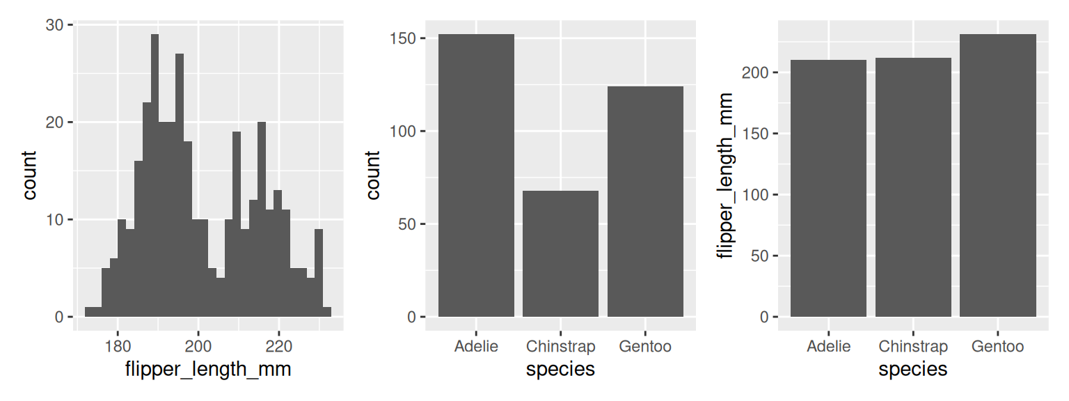
x <- ggplot(penguins) + geom_bar(aes(x=flipper_length_mm),stat="bin")
y <- ggplot(penguins) + geom_bar(aes(x=species),stat="count")
z <- ggplot(penguins) + geom_bar(aes(x=species,y=flipper_length_mm),stat="identity")
wrap_plots(x,y,z,nrow=1)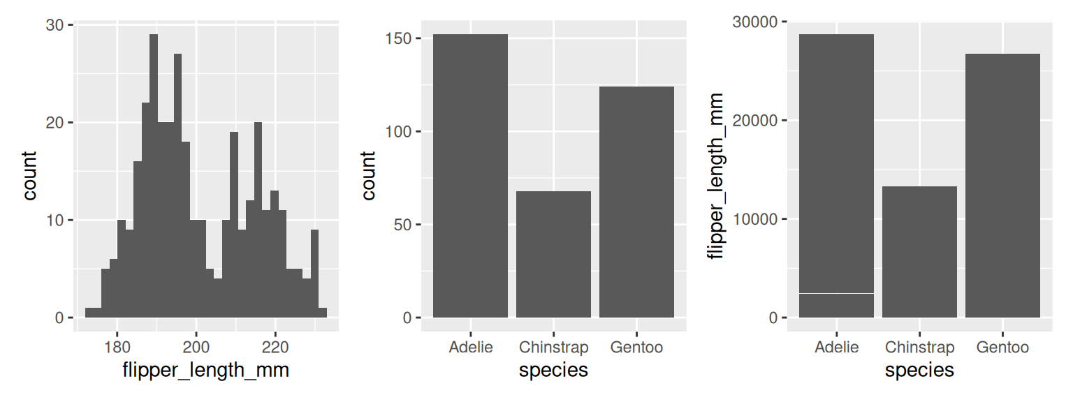
NBIS, SciLifeLab
19-May-2025

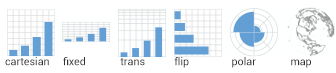
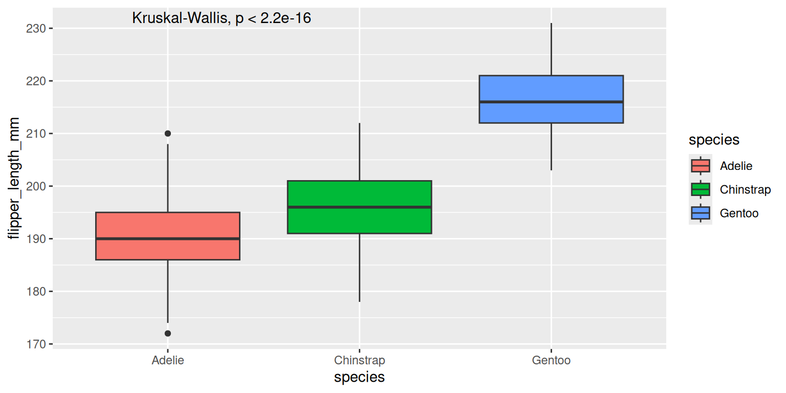
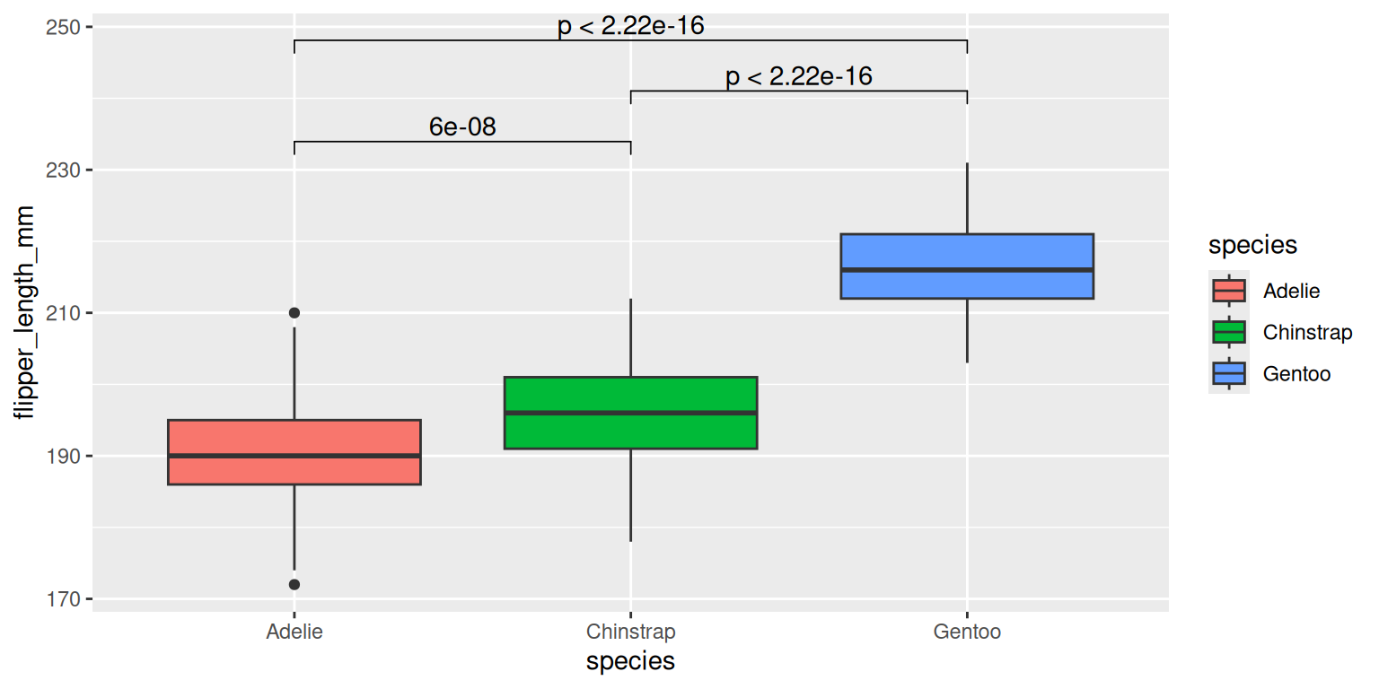
coord_cartesian(xlim=c(2,8)) for zooming incoord_map for controlling limits on mapscoord_polarstat_compare_means() from the package ggpubr.stat_compare_means() from the package ggpubr.p <- p + theme(
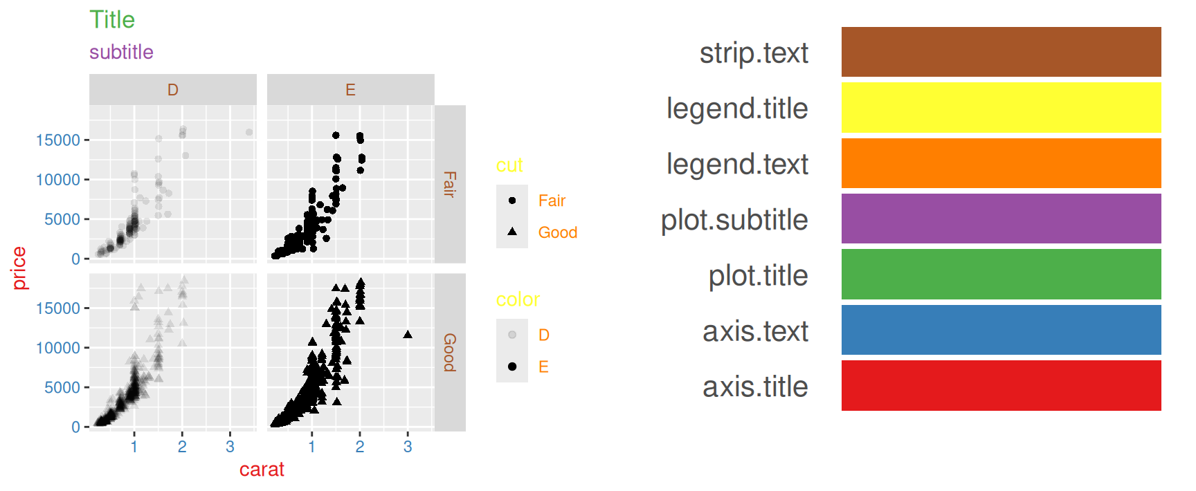
axis.title=element_text(color="#e41a1c"),
axis.text=element_text(color="#377eb8"),
plot.title=element_text(color="#4daf4a"),
plot.subtitle=element_text(color="#984ea3"),
legend.text=element_text(color="#ff7f00"),
legend.title=element_text(color="#ffff33"),
strip.text=element_text(color="#a65628")
)
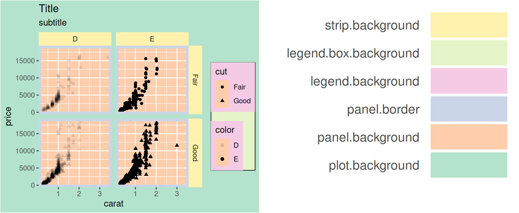
p <- p + theme(
    plot.background=element_rect(fill="#b3e2cd"),
    panel.background=element_rect(fill="#fdcdac"),
    panel.border=element_rect(fill=NA,color="#cbd5e8",size=3),
    legend.background=element_rect(fill="#f4cae4"),
    legend.box.background=element_rect(fill="#e6f5c9"),
    strip.background=element_rect(fill="#fff2ae")
)
newtheme <- theme_bw() + theme(
  axis.ticks=element_blank(),
  panel.background=element_rect(fill="white"),
  panel.grid.minor=element_blank(),
  panel.grid.major.x=element_blank(),
  panel.grid.major.y=element_line(size=0.3,color="grey90"),
  panel.border=element_blank(),
  legend.position="top",
  legend.justification="right"
)Refer to patchwork documentation. Some notable alternatives are ggpubr and cowplot.