Spatial transcriptomics
Adapted from tutorials by Giovanni Palla (https://scanpy-tutorials.readthedocs.io/en/latest/spatial/integration-scanorama.html) and Carlos Talavera-López (https://docs.scvi-tools.org/en/latest/tutorials/notebooks/stereoscope_heart_LV_tutorial.html)
OBS! For this tutorial you must create and use a new conda environment python_spatial. The recipe can be found at: https://raw.githubusercontent.com/NBISweden/workshop-scRNAseq/master/labs/environment_python_spatial.yml
Spatial transcriptomic data with the Visium platform is in many ways similar to scRNAseq data. It contains UMI counts for 5-20 cells instead of single cells, but is still quite sparse in the same way as scRNAseq data is, but with the additional information about spatial location in the tissue.
Here we will first run quality control in a similar manner to scRNAseq data, then QC filtering, dimensionality reduction, integration and clustering. Then we will use scRNAseq data from mouse cortex to run LabelTransfer to predict celltypes in the Visium spots.
We will use two Visium spatial transcriptomics dataset of the mouse brain (Sagittal), which are publicly available from the 10x genomics website. Note, that these dataset have already been filtered for spots that does not overlap with the tissue.
Load packages
import warnings
warnings.simplefilter(action='ignore', category=FutureWarning)

import scanpy as sc
import anndata as an
import pandas as pd
import numpy as np
import matplotlib as mpl
import matplotlib.pyplot as plt
import seaborn as sns
import scanorama
#sc.logging.print_versions() # gives errror!!
sc.set_figure_params(facecolor="white", figsize=(8, 8))
sc.settings.verbosity = 3
Load ST data
The function datasets.visium_sge() downloads the dataset from 10x genomics and returns an AnnData object that contains counts, images and spatial coordinates. We will calculate standards QC metrics with pp.calculate_qc_metrics and visualize them.
When using your own Visium data, use Scanpy's read_visium() function to import it.
adata_anterior = sc.datasets.visium_sge(
    sample_id="V1_Mouse_Brain_Sagittal_Anterior"
)
adata_posterior = sc.datasets.visium_sge(
    sample_id="V1_Mouse_Brain_Sagittal_Posterior"
)
adata_anterior.var_names_make_unique()
adata_posterior.var_names_make_unique()
To make sure that both images are included in the merged object, use uns_merge="unique".
# merge into one dataset
library_names = ["V1_Mouse_Brain_Sagittal_Anterior", "V1_Mouse_Brain_Sagittal_Posterior"]

adata = adata_anterior.concatenate(
    adata_posterior,
    batch_key="library_id",
    uns_merge="unique",
    batch_categories=library_names
)
adata
As you can see, we now have the slot spatial in obsm, which contains the spatial information from the Visium platform.
Quality control
Similar to scRNAseq we use statistics on number of counts, number of features and percent mitochondria for quality control.
# add info on mitochondrial and hemoglobin genes to the objects.
adata.var['mt'] = adata.var_names.str.startswith('mt-')
adata.var['hb'] = adata.var_names.str.contains(("^Hb.*-"))

sc.pp.calculate_qc_metrics(adata, qc_vars=['mt','hb'], percent_top=None, log1p=False, inplace=True)
sc.pl.violin(adata, ['n_genes_by_counts', 'total_counts', 'pct_counts_mt', 'pct_counts_hb'],
             jitter=0.4, groupby = 'library_id', rotation= 45)
We can also plot the same data onto the tissue section.
In scanpy, this is a bit tricky when you have multiple sections, as you would have to subset and plot them separately.
# need to plot the two sections separately and specify the library_id

for library in library_names:
    sc.pl.spatial(adata[adata.obs.library_id == library,:], library_id=library, color = ["total_counts", "n_genes_by_counts",'pct_counts_mt', 'pct_counts_hb'])
As you can see, the spots with low number of counts/features and high mitochondrial content is mainly towards the edges of the tissue. It is quite likely that these regions are damaged tissue. You may also see regions within a tissue with low quality if you have tears or folds in your section.
But remember, for some tissue types, the amount of genes expressed and proportion mitochondria may also be a biological features, so bear in mind what tissue you are working on and what these features mean.
Filter
Select all spots with less than 25% mitocondrial reads, less than 20% hb-reads and 1000 detected genes. You must judge for yourself based on your knowledge of the tissue what are appropriate filtering criteria for your dataset.
keep = (adata.obs['pct_counts_hb'] < 20) & (adata.obs['pct_counts_mt'] < 25) & (adata.obs['n_genes_by_counts'] > 1000)
print(sum(keep))

adata = adata[keep,:]
And replot onto tissue sections.
for library in library_names:
    sc.pl.spatial(adata[adata.obs.library_id == library,:], library_id=library, color = ["total_counts", "n_genes_by_counts",'pct_counts_mt', 'pct_counts_hb'])
Top expressed genes
sc.pl.highest_expr_genes(adata, n_top=20)
As you can see, the mitochondrial genes are among the top expressed. Also the lncRNA gene Bc1 (brain cytoplasmic RNA 1). Also one hemoglobin gene.
Filter genes
We will remove the Bc1 gene, hemoglobin genes (blood contamination) and the mitochondrial genes.
mito_genes = adata.var_names.str.startswith('mt-')
hb_genes = adata.var_names.str.contains('^Hb.*-')

remove = np.add(mito_genes, hb_genes)
remove[adata.var_names == "Bc1"] = True
keep = np.invert(remove)
print(sum(remove))

adata = adata[:,keep]

print(adata.n_obs, adata.n_vars)
Analysis
As we have two sections, we will select variable genes with batch_key="library_id" and then take the union of variable genes for further analysis. The idea is to avoid including batch specific genes in the analysis.
# save the counts to a separate object for later, we need the normalized counts in raw for DEG dete
counts_adata = adata.copy()

sc.pp.normalize_total(adata, inplace=True)
sc.pp.log1p(adata)
# take 1500 variable genes per batch and then use the union of them.
sc.pp.highly_variable_genes(adata, flavor="seurat", n_top_genes=1500, inplace=True, batch_key="library_id")

# subset for variable genes
adata.raw = adata
adata = adata[:,adata.var.highly_variable_nbatches > 0]

# scale data
sc.pp.scale(adata)
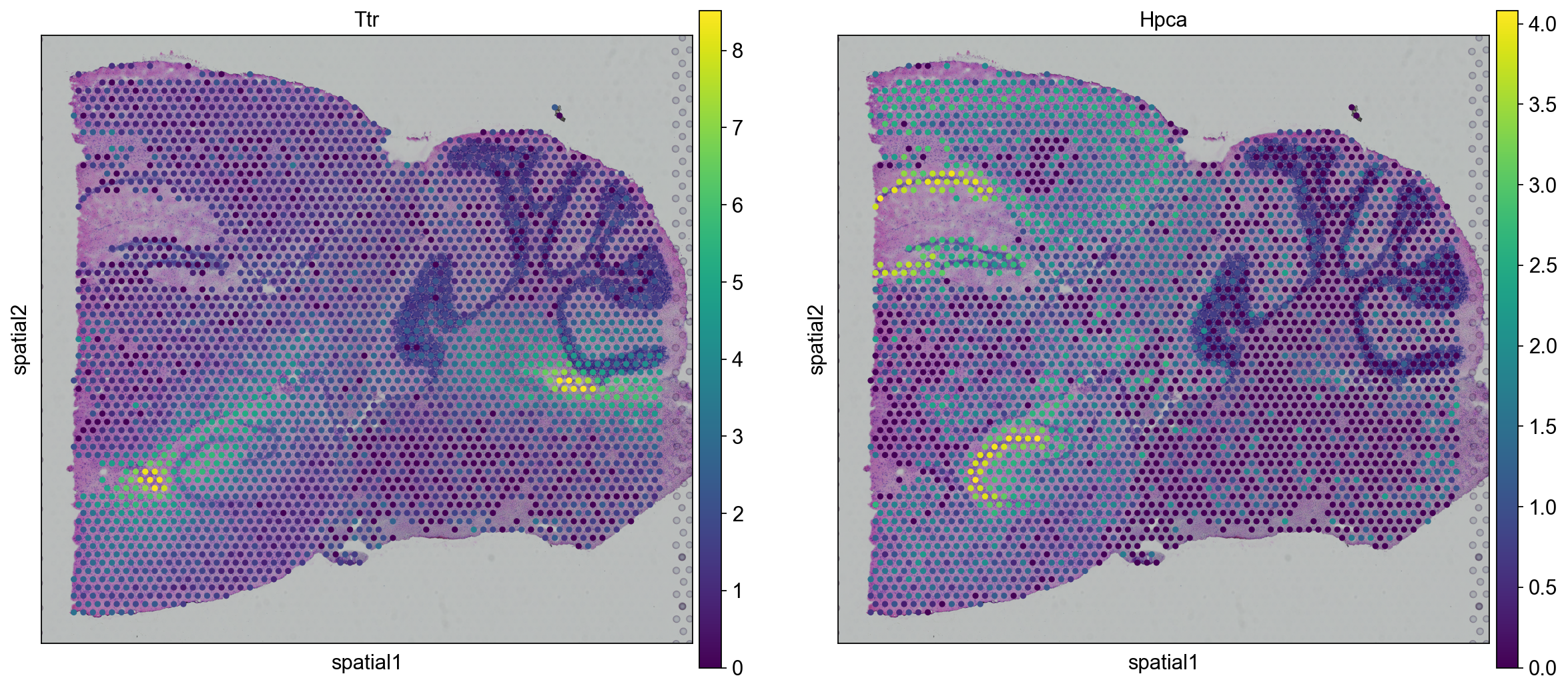
Now we can plot gene expression of individual genes, the gene Hpca is a strong hippocampal marker and Ttr is a marker of the choroid plexus.
for library in library_names:
    sc.pl.spatial(adata[adata.obs.library_id == library,:], library_id=library, color = ["Ttr", "Hpca"])
Dimensionality reduction and clustering
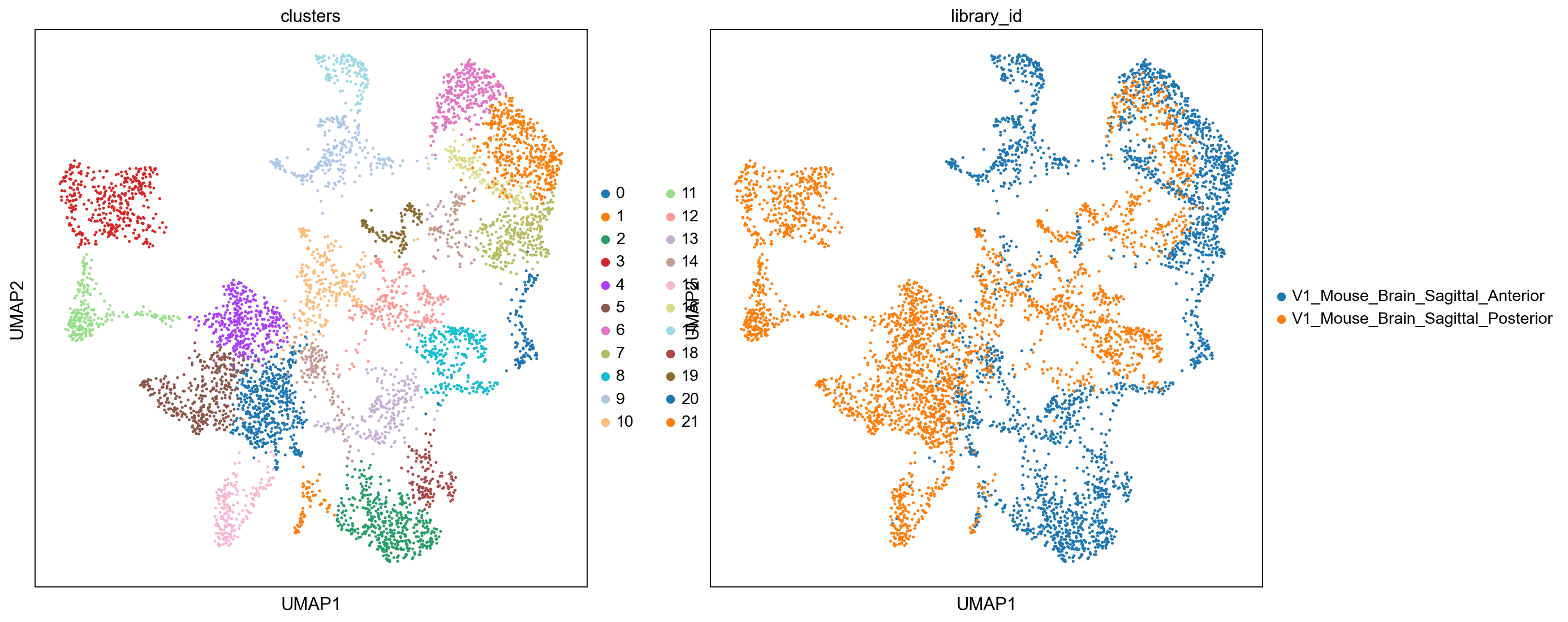
We can then now run dimensionality reduction and clustering using the same workflow as we use for scRNA-seq analysis.
sc.pp.neighbors(adata)
sc.tl.umap(adata)
sc.tl.leiden(adata, key_added="clusters")
Dimensionality reduction and clustering
We can then now run dimensionality reduction and clustering using the same workflow as we use for scRNA-seq analysis.
sc.pl.umap(
    adata, color=["clusters", "library_id"], palette=sc.pl.palettes.default_20
)
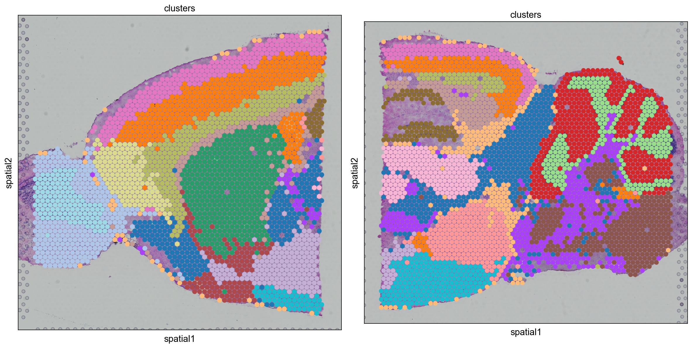
As we are plotting the two sections separately, we need to make sure that they get the same colors by fetching cluster colors from a dict.
clusters_colors = dict(
    zip([str(i) for i in range(len(adata.obs.clusters.cat.categories))], adata.uns["clusters_colors"])
)

fig, axs = plt.subplots(1, 2, figsize=(15, 10))

for i, library in enumerate(
    ["V1_Mouse_Brain_Sagittal_Anterior", "V1_Mouse_Brain_Sagittal_Posterior"]
):
    ad = adata[adata.obs.library_id == library, :].copy()
    sc.pl.spatial(
        ad,
        img_key="hires",
        library_id=library,
        color="clusters",
        size=1.5,
        palette=[
            v
            for k, v in clusters_colors.items()
            if k in ad.obs.clusters.unique().tolist()
        ],
        legend_loc=None,
        show=False,
        ax=axs[i],
    )

plt.tight_layout()
Integration
Quite often there are strong batch effects between different ST sections, so it may be a good idea to integrate the data across sections.
We will do a similar integration as in the Data Integration lab, here we will use Scanorama for integration.
adatas = {}
for batch in library_names:
    adatas[batch] = adata[adata.obs['library_id'] == batch,]

adatas
import scanorama

#convert to list of AnnData objects
adatas = list(adatas.values())

# run scanorama.integrate
scanorama.integrate_scanpy(adatas, dimred = 50)


# Get all the integrated matrices.
scanorama_int = [ad.obsm['X_scanorama'] for ad in adatas]

# make into one matrix.
all_s = np.concatenate(scanorama_int)
print(all_s.shape)

# add to the AnnData object
adata.obsm["Scanorama"] = all_s
adata
Then we run dimensionality reduction and clustering as before.
sc.pp.neighbors(adata, use_rep="Scanorama")
sc.tl.umap(adata)
sc.tl.leiden(adata, key_added="clusters")
sc.pl.umap(
    adata, color=["clusters", "library_id"], palette=sc.pl.palettes.default_20
)
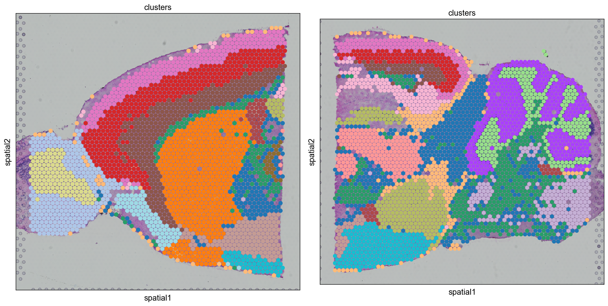
As we have new clusters, we again need to make a new dict for cluster colors
clusters_colors = dict(
    zip([str(i) for i in range(len(adata.obs.clusters.cat.categories))], adata.uns["clusters_colors"])
)


fig, axs = plt.subplots(1, 2, figsize=(15, 10))

for i, library in enumerate(
    ["V1_Mouse_Brain_Sagittal_Anterior", "V1_Mouse_Brain_Sagittal_Posterior"]
):
    ad = adata[adata.obs.library_id == library, :].copy()
    sc.pl.spatial(
        ad,
        img_key="hires",
        library_id=library,
        color="clusters",
        size=1.5,
        palette=[
            v
            for k, v in clusters_colors.items()
            if k in ad.obs.clusters.unique().tolist()
        ],
        legend_loc=None,
        show=False,
        ax=axs[i],
    )

plt.tight_layout()
Do you see any differences between the integrated and non-integrated clusering? Judge for yourself, which of the clusterings do you think looks best? As a reference, you can compare to brain regions in the Allen brain atlas.
Identification of Spatially Variable Features
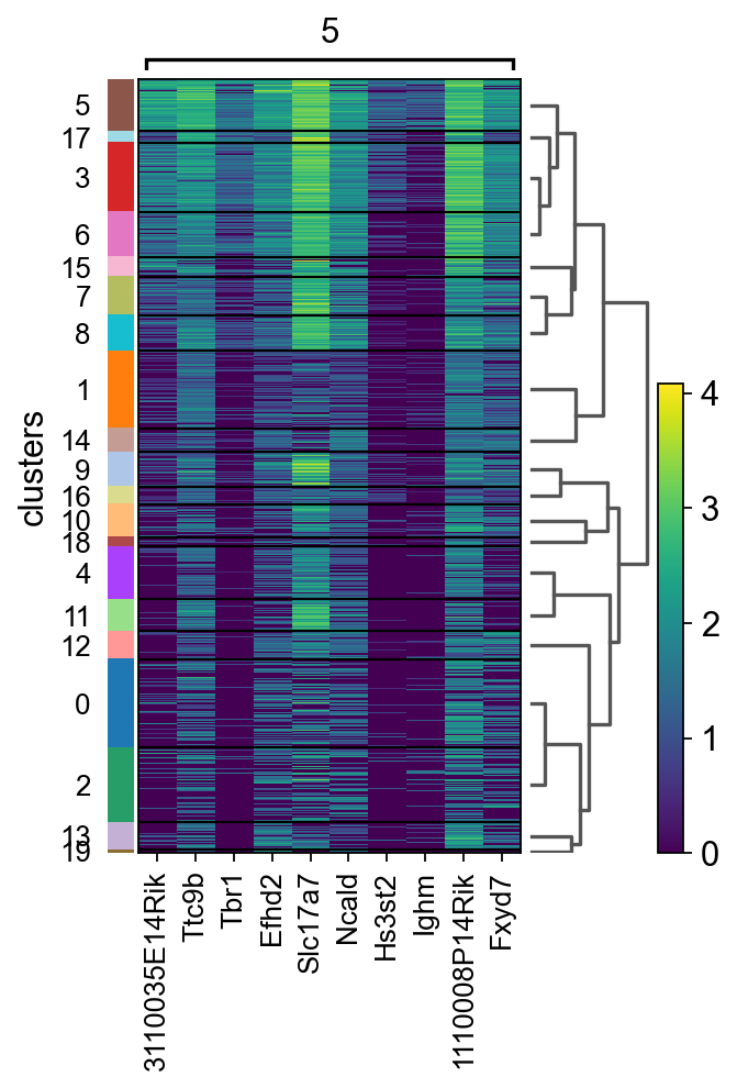
There are two main workflows to identify molecular features that correlate with spatial location within a tissue. The first is to perform differential expression based on spatially distinct clusters, the other is to find features that are have spatial patterning without taking clusters or spatial annotation into account.
First, we will do differential expression between clusters just as we did for the scRNAseq data before.
# run t-test
sc.tl.rank_genes_groups(adata, "clusters", method="wilcoxon")
# plot as heatmap for cluster5 genes
sc.pl.rank_genes_groups_heatmap(adata, groups="5", n_genes=10, groupby="clusters")
# plot onto spatial location
top_genes = sc.get.rank_genes_groups_df(adata, group='5',log2fc_min=0)['names'][:3]


for library in ["V1_Mouse_Brain_Sagittal_Anterior", "V1_Mouse_Brain_Sagittal_Posterior"]:
    sc.pl.spatial(adata[adata.obs.library_id == library,:], library_id=library, color = top_genes)
We use SpatialDE Svensson et al., a Gaussian process-based statistical framework that aims to identify spatially variable genes.
OBS! Takes a long time to run, so skip this step for now!
# import SpatialDE

# #First, we convert normalized counts and coordinates to pandas dataframe, needed for inputs to spatialDE.
# counts = pd.DataFrame(adata.X.todense(), columns=adata.var_names, index=adata.obs_names)
# coord = pd.DataFrame(adata.obsm['spatial'], columns=['x_coord', 'y_coord'], index=adata.obs_names)
# results = SpatialDE.run(coord, counts)

# #We concatenate the results with the DataFrame of annotations of variables: `adata.var`.
# results.index = results["g"]
# adata.var = pd.concat([adata.var, results.loc[adata.var.index.values, :]], axis=1)

# #Then we can inspect significant genes that varies in space and visualize them with `sc.pl.spatial` function.
# results.sort_values("qval").head(10)
Single cell data
We can use a scRNA-seq dataset as a referenced to predict the proportion of different celltypes in the Visium spots.
Keep in mind that it is important to have a reference that contains all the celltypes you expect to find in your spots. Ideally it should be a scRNAseq reference from the exact same tissue.
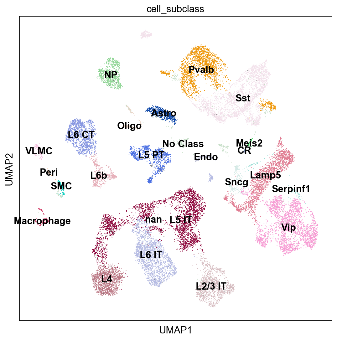
We will use a reference scRNA-seq dataset of ~14,000 adult mouse cortical cell taxonomy from the Allen Institute, generated with the SMART-Seq2 protocol.
Conveniently, you can also download the pre-processed dataset in h5ad format from here. Here with bash code:
%%bash

FILE="./data/spatial/adata_processed_sc.h5ad"

if [ -e $FILE ]
then
   echo "File $FILE is downloaded."
else
   echo "Downloading $FILE"
   mkdir -p data/spatial
   wget -O data/spatial/adata_processed_sc.h5ad https://hmgubox.helmholtz-muenchen.de/f/4ef254675e2a41f89835/?dl=1
fi
adata_cortex=sc.read_h5ad("data/spatial/adata_processed_sc.h5ad")
sc.pl.umap(adata_cortex, color="cell_subclass", legend_loc = 'on data')
adata_cortex.obs.cell_subclass.value_counts()
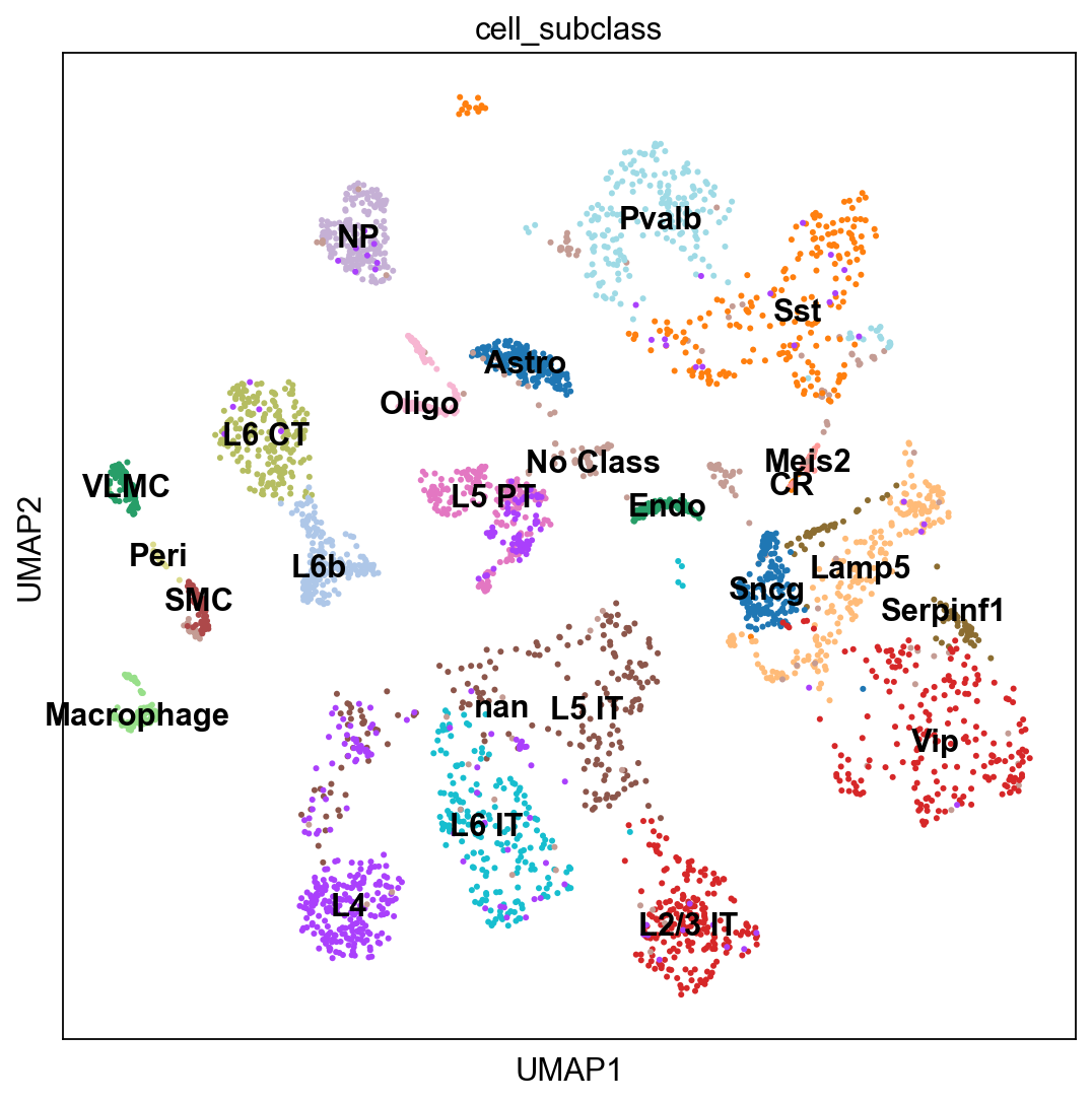
For speed, and for a more fair comparison of the celltypes, we will subsample all celltypes to a maximum of 200 cells per class (subclass).
target_cells = 200

adatas2 = [adata_cortex[adata_cortex.obs.cell_subclass == clust] for clust in adata_cortex.obs.cell_subclass.cat.categories]

for dat in adatas2:
    if dat.n_obs > target_cells:
         sc.pp.subsample(dat, n_obs=target_cells)

adata_cortex = adatas2[0].concatenate(*adatas2[1:])

adata_cortex.obs.cell_subclass.value_counts()
sc.pl.umap(
    adata_cortex, color=["cell_class", "cell_subclass","donor_genotype","dissected_region"], palette=sc.pl.palettes.default_20
)
sc.pl.umap(adata_cortex, color="cell_subclass", legend_loc = 'on data')
Subset ST for cortex
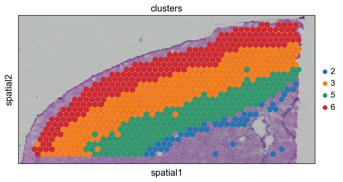
Since the scRNAseq dataset was generated from the mouse cortex, we will subset the visium dataset in order to select mainly the spots part of the cortex. Note that the integration can also be performed on the whole brain slice, but it would give rise to false positive cell type assignments and and therefore it should be interpreted with more care.
OBS! For deconvolution we will need the counts data, so we will subset from the counts_adata object that we created earlier.
lib_a = "V1_Mouse_Brain_Sagittal_Anterior"

counts_adata.obs['clusters'] = adata.obs.clusters

adata_anterior_subset = counts_adata[
    (counts_adata.obs.library_id == lib_a)
    & (counts_adata.obsm["spatial"][:, 1] < 6000), :
].copy()

# select also the cortex clusters
adata_anterior_subset = adata_anterior_subset[adata_anterior_subset.obs.clusters.isin(['2','3','5','6']),:]
# plot to check that we have the correct regions

sc.pl.spatial(
    adata_anterior_subset,
    img_key="hires",
    library_id = lib_a,
    color=['clusters'],
    size=1.5
)
Deconvolution
Deconvolution is a method to estimate the abundance (or proportion) of different celltypes in a bulkRNAseq dataset using a single cell reference. As the Visium data can be seen as a small bulk, we can both use methods for traditional bulkRNAseq as well as methods especially developed for Visium data. Some methods for deconvolution are DWLS, cell2location, Tangram, Stereoscope, RCTD, SCDC and many more.
Here, we will use deconvolution with Stereoscope implemented in the SCVI-tools package. To read more about Stereoscope please check out this github page (https://github.com/almaan/stereoscope)
Select genes for deconvolution
Most deconvolution methods does a prior gene selection and there are different options that are used:
- Use variable genes in the SC data.
- Use variable genes in both SC and ST data
- DE genes between clusters in the SC data.
In this case we will use top DEG genes per cluster, so first we have to run DEG detection on the scRNAseq data.
sc.tl.rank_genes_groups(adata_cortex, 'cell_subclass', method = "t-test", n_genes=100)
sc.pl.rank_genes_groups_dotplot(adata_cortex, n_genes=3)
sc.tl.filter_rank_genes_groups(adata_cortex, min_fold_change=1)

genes = sc.get.rank_genes_groups_df(adata_cortex, group = None)
genes
deg = genes.names.unique().tolist()
print(len(deg))
# check that the genes are also present in the ST data


deg = np.intersect1d(deg,adata_anterior_subset.var.index).tolist()
print(len(deg))
Train the model
First, train the model using scRNAseq data.
Stereoscope requires the data to be in counts, earlier in this tutorial we saved the spatial counts in a separate object counts_adata.
However, the single cell dataset that we dowloaded only has the lognormalized data in the adata.X slot, hence we will have to recalculate the count matrix.
# first do exponent and subtract pseudocount
E = np.exp(adata_cortex.X)-1
n = np.sum(E,1)
print(np.min(n), np.max(n))
# all sums to 1.7M
factor = np.mean(n)
nC = np.array(adata_cortex.obs.total_counts) # true number of counts
scaleF = nC/factor
C = E * scaleF[:,None]
C = C.astype("int")
sc_adata = adata_cortex.copy()
sc_adata.X = C
Setup the anndata, the implementation requires the counts matrix to be in the "counts" layer as a copy.
import scvi
#from scvi.data import register_tensor_from_anndata
from scvi.external import RNAStereoscope, SpatialStereoscope

# add counts layer
sc_adata.layers["counts"] = sc_adata.X.copy()

# subset for the selected genes
sc_adata = sc_adata[:, deg].copy()

# create stereoscope object
RNAStereoscope.setup_anndata(sc_adata, layer = "counts", labels_key = "cell_subclass")
# the model is saved to a file, so if is slow to run, you can simply reload it from disk by setting train = False

train = True
if train:
    sc_model = RNAStereoscope(sc_adata)
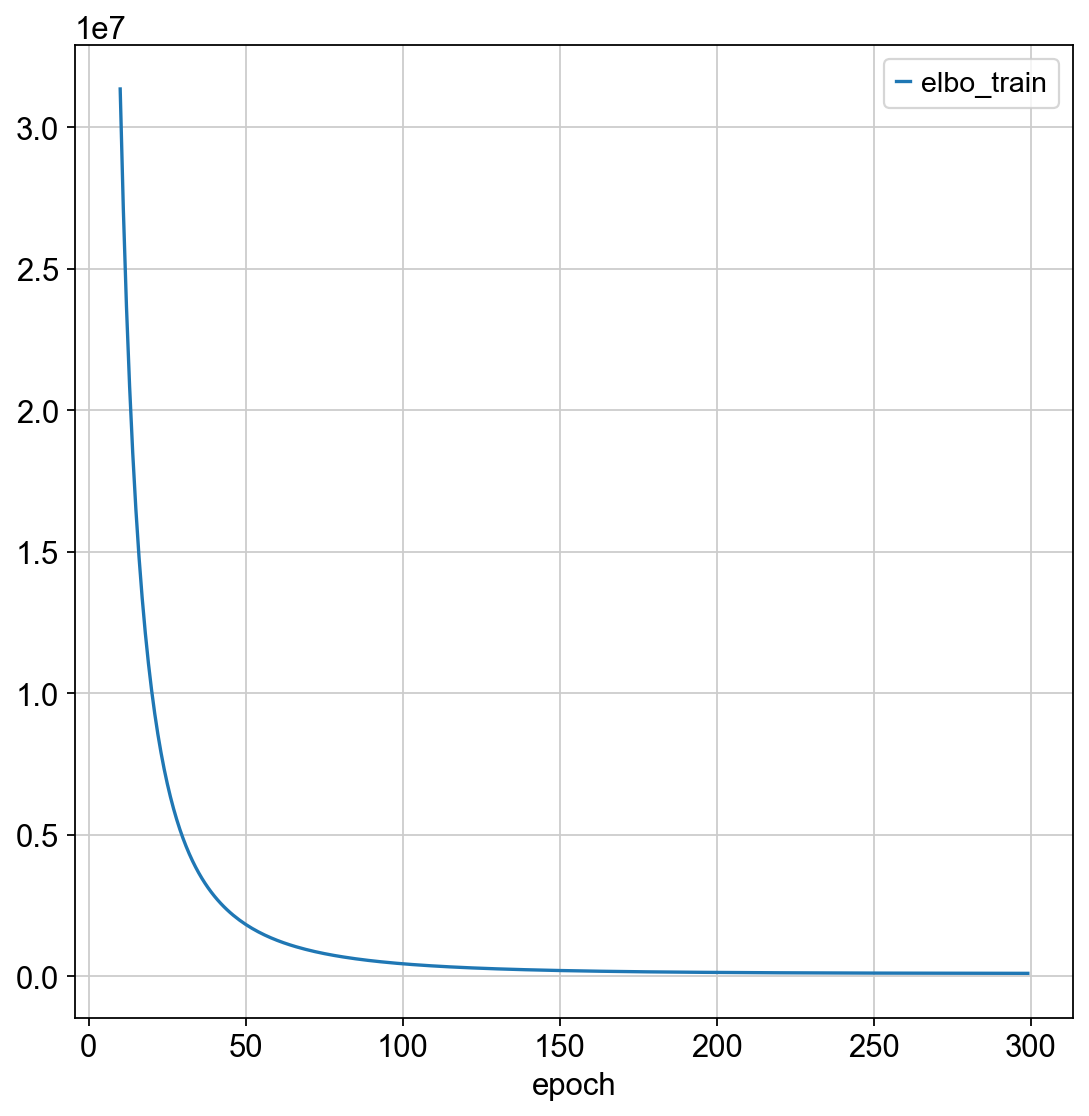
    sc_model.train(max_epochs = 300)
    sc_model.history["elbo_train"][10:].plot()
    sc_model.save("./data/spatial/scmodel", overwrite=True)
else:
    sc_model = RNAStereoscope.load("./data/spatial/scmodel", sc_adata)
    print("Loaded RNA model from file!")
Predict propritions on the spatial data
First create a new st object with the correct genes and counts as a layer.
st_adata = adata_anterior_subset.copy()

st_adata.layers["counts"] = st_adata.X.copy()
st_adata = st_adata[:, deg].copy()

SpatialStereoscope.setup_anndata(st_adata, layer="counts")
train=True
if train:
    spatial_model = SpatialStereoscope.from_rna_model(st_adata, sc_model)
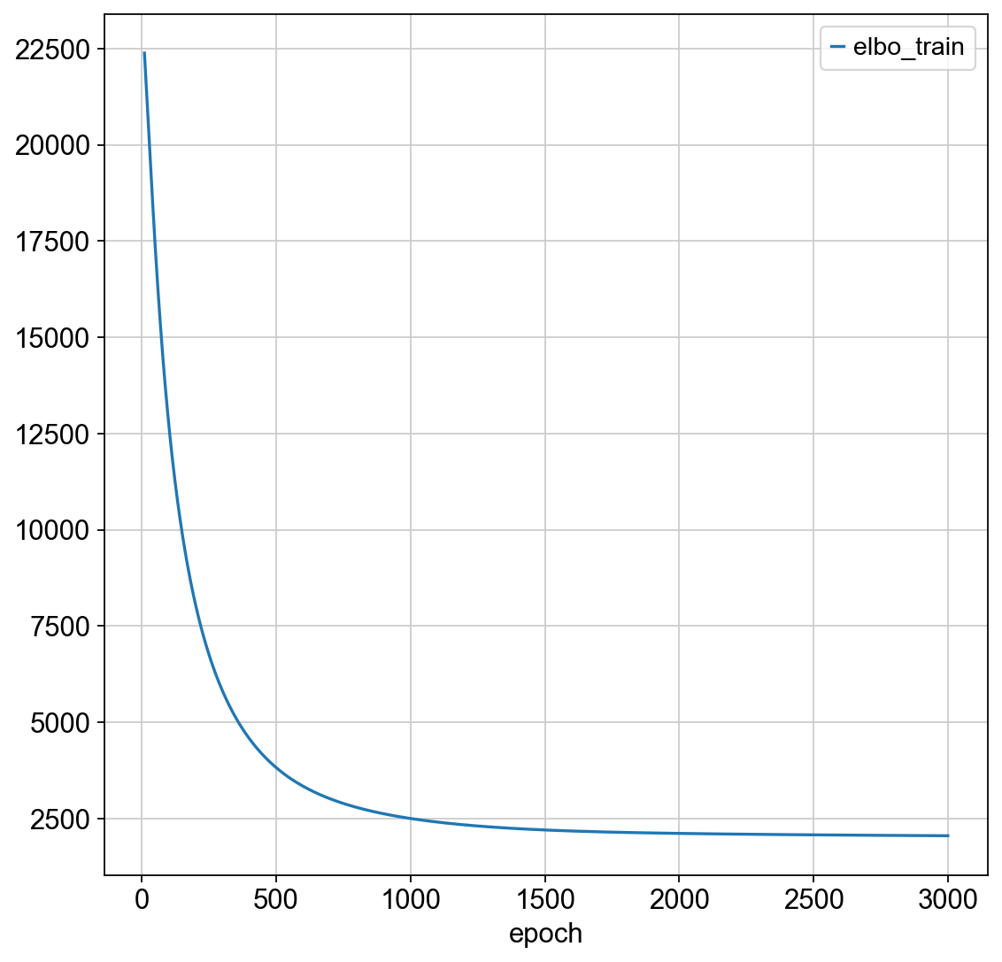
    spatial_model.train(max_epochs = 3000)
    spatial_model.history["elbo_train"][10:].plot()
    spatial_model.save("./data/spatial/stmodel", overwrite = True)
else:
    spatial_model = SpatialStereoscope.load("./data/spatial/stmodel", st_adata)
    print("Loaded Spatial model from file!")
Get the results from the model, also put them in the .obs slot.
st_adata.obsm["deconvolution"] = spatial_model.get_proportions()

# also copy to the obsm data frame
for ct in st_adata.obsm["deconvolution"].columns:
    st_adata.obs[ct] = st_adata.obsm["deconvolution"][ct]
We are then able to explore how cell types in the scRNA-seq dataset are predicted onto the visium dataset. Let's first visualize the neurons cortical layers.
sc.pl.spatial(
    st_adata,
    img_key="hires",
    color=["L2/3 IT", "L4", "L5 PT", "L6 CT"],
    library_id=lib_a,
    size=1.5,
    ncols=2
)
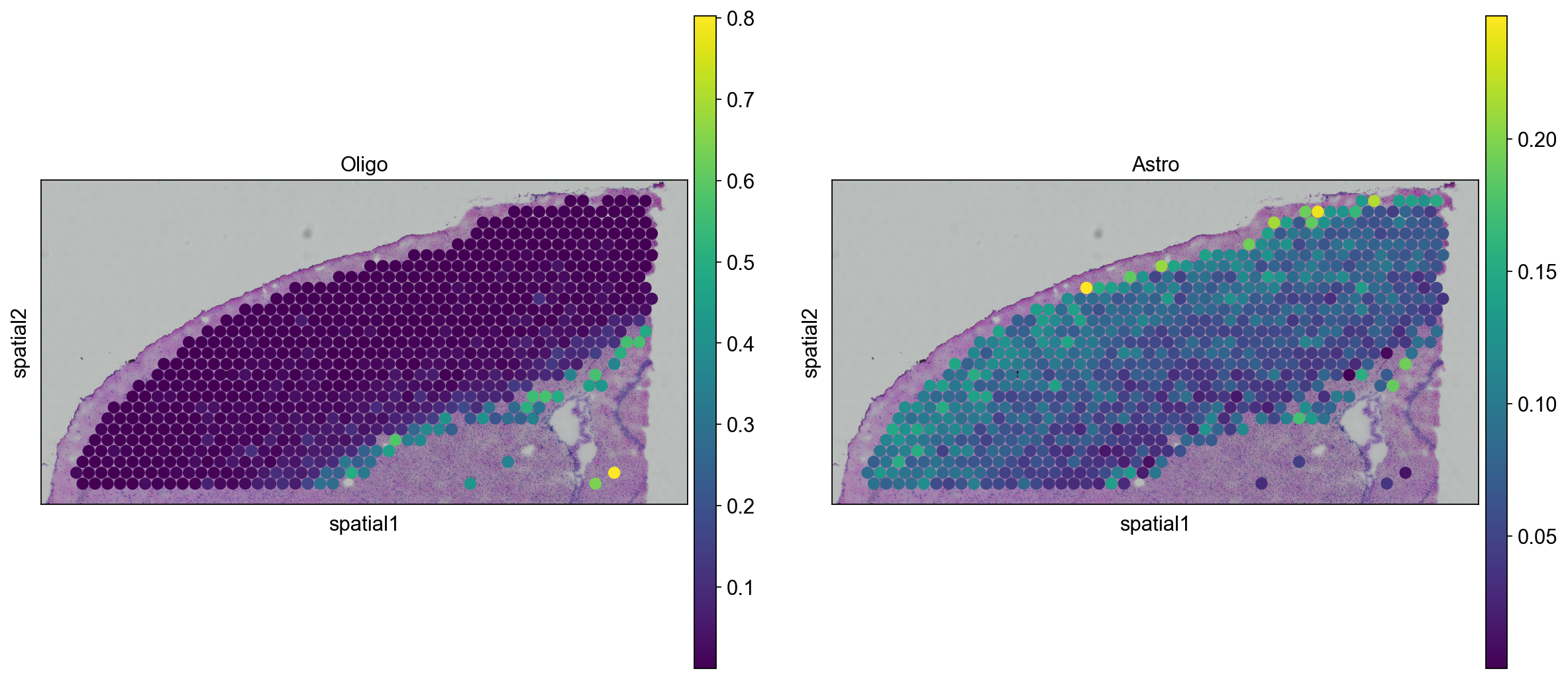
We can go ahead an visualize astrocytes and oligodendrocytes as well.
sc.pl.spatial(
    st_adata, img_key="hires", color=["Oligo", "Astro"], size=1.5, library_id = lib_a
)
We can also visualize the scores per cluster in ST data
sc.pl.violin(st_adata, ["L2/3 IT", "L6 CT","Oligo","Astro"],
            jitter=0.4, groupby = 'clusters', rotation= 45)
Keep in mind that the deconvolution results are just predictions, depending on how well your scRNAseq data covers the celltypes that are present in the ST data and on how parameters, gene selection etc. are tuned you may get different results.
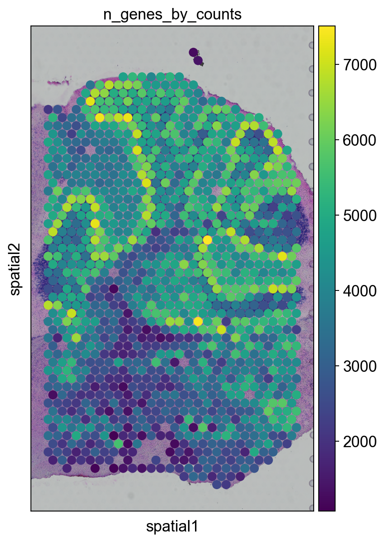
lib_p = "V1_Mouse_Brain_Sagittal_Posterior"

adata_subregion = adata[
    (adata.obs.library_id == lib_p)
    & (adata.obsm["spatial"][:, 0] > 6500),
    :,
].copy()
sc.pl.spatial(
    adata_subregion,
    img_key="hires",
    library_id = lib_p,
    color=['n_genes_by_counts'],
    size=1.5
)


