Scanpy: Differential expression
Once we have done clustering, let's compute a ranking for the highly differential genes in each cluster.
Differential expression is performed with the function rank_genes_group. The default method to compute differential expression is the t-test_overestim_var. Other implemented methods are: logreg, t-test and wilcoxon.
By default, the .raw attribute of AnnData is used in case it has been initialized, it can be changed by setting use_raw=False.
OBS! Note that by default the method uses setting n_genes=100, and will only report top 100 genes.
The clustering with resolution 0.6 seems to give a reasonable number of clusters, so we will use that clustering for all DE tests.
First, let's import libraries and fetch the clustered data from the previous lab.
import numpy as np
import pandas as pd
import scanpy as sc
import matplotlib.pyplot as plt

sc.settings.verbosity = 2             # verbosity: errors (0), warnings (1), info (2), hints (3)
sc.logging.print_versions()
sc.settings.set_figure_params(dpi=80)
Read in the clustered data object.
adata = sc.read_h5ad('./data/scanpy_clustered_3pbmc.h5ad')
print(adata.shape)
print(adata.raw.shape)
T-test
sc.tl.rank_genes_groups(adata, 'louvain_0.6', method='t-test', key_added = "t-test")
sc.pl.rank_genes_groups(adata, n_genes=25, sharey=False, key = "t-test")

# results are stored in the adata.uns["t-test"] slot
adata
T-test overestimated_variance
sc.tl.rank_genes_groups(adata, 'louvain_0.6', method='t-test_overestim_var', key_added = "t-test_ov")
sc.pl.rank_genes_groups(adata, n_genes=25, sharey=False, key = "t-test_ov")

Wilcoxon rank-sum
The result of a Wilcoxon rank-sum (Mann-Whitney-U) test is very similar. We recommend using the latter in publications, see e.g., Sonison & Robinson (2018). You might also consider much more powerful differential testing packages like MAST, limma, DESeq2 and, for python, the recent diffxpy.
sc.tl.rank_genes_groups(adata, 'louvain_0.6', method='wilcoxon', key_added = "wilcoxon")
sc.pl.rank_genes_groups(adata, n_genes=25, sharey=False, key="wilcoxon")

Logistic regression test
As an alternative, let us rank genes using logistic regression. For instance, this has been suggested by Natranos et al. (2018). The essential difference is that here, we use a multi-variate appraoch whereas conventional differential tests are uni-variate. Clark et al. (2014) has more details.
sc.tl.rank_genes_groups(adata, 'louvain_0.6', method='logreg',key_added = "logreg")
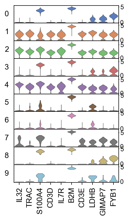
sc.pl.rank_genes_groups(adata, n_genes=25, sharey=False, key = "logreg")

Compare genes
Take the top 100 DE genes for cluster0 with each test and compare the overlap.
#compare cluster1 genes, only stores top 100 by default

wc = adata.uns['wilcoxon']['names']['0']
tt = adata.uns['t-test']['names']['0']
tt_ov = adata.uns['t-test_ov']['names']['0']
lr = adata.uns['logreg']['names']['0']

from matplotlib_venn import venn3

venn3([set(wc),set(tt),set(tt_ov)], ('Wilcox','T-test','T-test_ov') )
plt.show()


venn3([set(wc),set(lr),set(tt_ov)], ('Wilcox','Logreg','T-test_ov') )
plt.show()

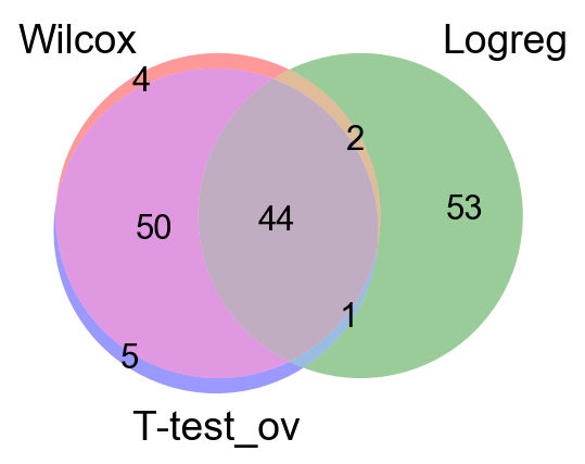
As you can see, the Wilcoxon test and the T-test with overestimated variance gives very similar result. Also the regular T-test has good overlap, while the Logistic regression gives quite different genes.
Visualization
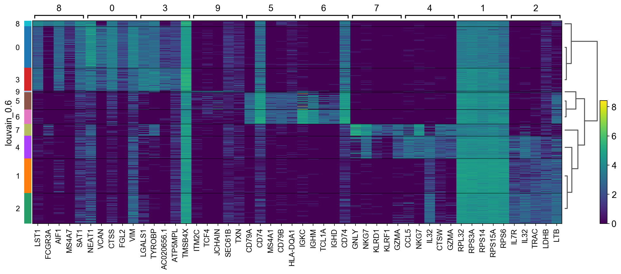
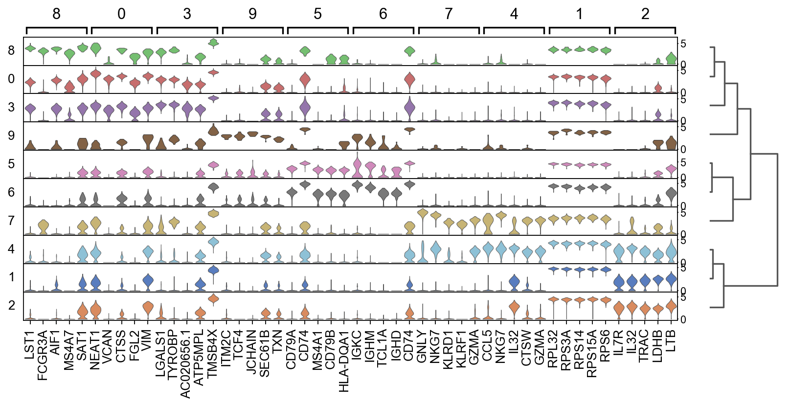
There are several ways to visualize the expression of top DE genes. Here we will plot top 5 genes per cluster from Wilcoxon test as heatmap, dotplot, violin plot or matrix.
sc.pl.rank_genes_groups_heatmap(adata, n_genes=5, key="wilcoxon", groupby="louvain_0.6", show_gene_labels=True)
sc.pl.rank_genes_groups_dotplot(adata, n_genes=5, key="wilcoxon", groupby="louvain_0.6")

sc.pl.rank_genes_groups_stacked_violin(adata, n_genes=5, key="wilcoxon", groupby="louvain_0.6")
sc.pl.rank_genes_groups_matrixplot(adata, n_genes=5, key="wilcoxon", groupby="louvain_0.6")

Compare specific clusters
We can also do pairwise comparisons of individual clusters on one vs many clusters.
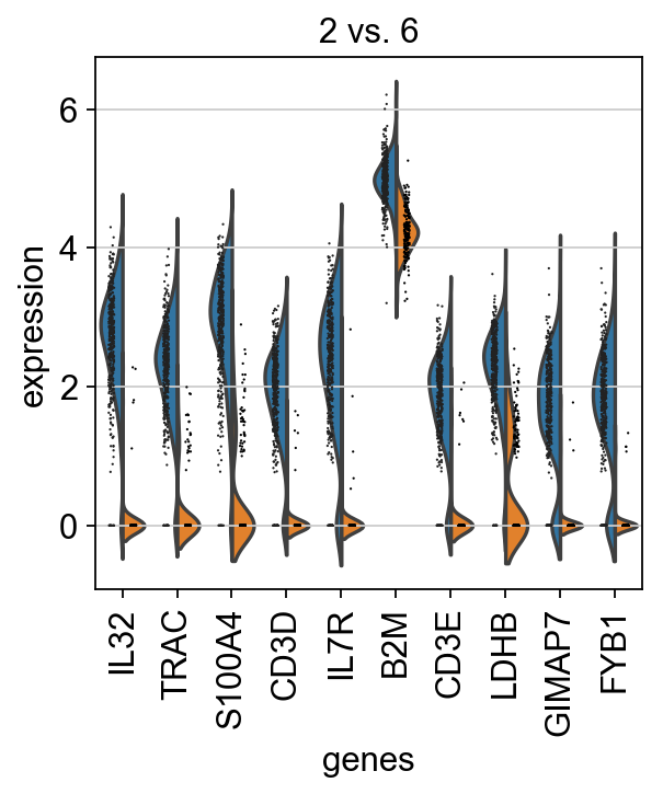
For instance, clusters 2 & 6 have very similar expression profiles.
sc.tl.rank_genes_groups(adata, 'louvain_0.6', groups=['2'], reference='6', method='wilcoxon')
sc.pl.rank_genes_groups(adata, groups=['2'], n_genes=20)

Plot as violins for those two groups.
sc.pl.rank_genes_groups_violin(adata, groups='2', n_genes=10)
# plot the same genes as violins across all the datasets.

# convert numpy.recarray to list
mynames = [x[0] for x in adata.uns['rank_genes_groups']['names'][:10]]
sc.pl.stacked_violin(adata, mynames, groupby = 'louvain_0.6')