Scanpy: Data integration
In this tutorial we will look at different ways of integrating multiple single cell RNA-seq datasets. We will explore two different methods to correct for batch effects across datasets. We will also look at a quantitative measure to assess the quality of the integrated data. Seurat uses the data integration method presented in Comprehensive Integration of Single Cell Data, while Scran and Scanpy use a mutual Nearest neighbour method (MNN). Below you can find a list of the most recent methods for single data integration:
| Markdown | Language | Library | Ref |
|---|---|---|---|
| CCA | R | Seurat | Cell |
| MNN | R/Python | Scater/Scanpy | Nat. Biotech. |
| Conos | R | conos | Nat. Methods |
| Scanorama | Python | scanorama | Nat. Biotech. |
import numpy as np
import pandas as pd
import scanpy as sc
import matplotlib.pyplot as plt

sc.settings.verbosity = 3             # verbosity: errors (0), warnings (1), info (2), hints (3)
sc.logging.print_versions()

sc.settings.set_figure_params(dpi=80)
%matplotlib inline
First need to load the QC filtered dataset and create individual adata objects per batch.
# Load the stored data object
save_file = './data/scanpy_dr_3pbmc.h5ad'
adata = sc.read_h5ad(save_file)
print(adata.X.shape)
As the stored AnnData object contains scaled data based on variable genes, we need to make a new object with the raw counts and normalized it again. Variable gene selection should not be performed on the scaled data object, only do normalization and log transformation before variable genes selection.
adata2 = sc.AnnData(X=adata.raw.X, var=adata.raw.var, obs = adata.obs)

sc.pp.normalize_per_cell(adata2, counts_per_cell_after=1e4)
sc.pp.log1p(adata2)
Detect variable genes
Variable genes can be detected across the full dataset, but then we run the risk of getting many batch-specific genes that will drive a lot of the variation. Or we can select variable genes from each batch separately to get only celltype variation. Here, we will do both as an example of how it can be done.
First we will select genes based on the full dataset.
#variable genes for the full dataset
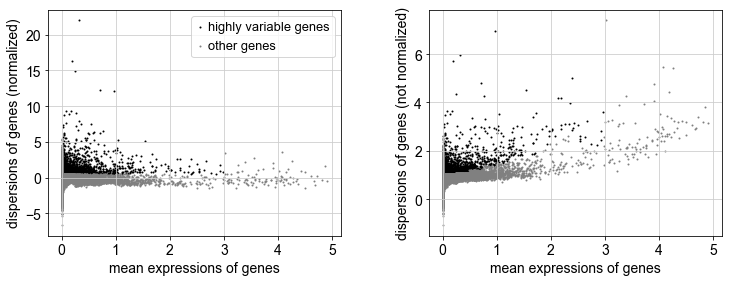
sc.pp.highly_variable_genes(adata2, min_mean=0.0125, max_mean=3, min_disp=0.5)
sc.pl.highly_variable_genes(adata2)
print("Highly variable genes: %d"%sum(adata2.var.highly_variable))
var_genes_all = adata2.var.highly_variable
Detect variable genes in each dataset separately using the batch_key parameter.
sc.pp.highly_variable_genes(adata2, min_mean=0.0125, max_mean=3, min_disp=0.5, batch_key = 'lib_prep')

print("Highly variable genes intersection: %d"%sum(adata2.var.highly_variable_intersection))

print("Number of batches where gene is variable:")
print(adata2.var.highly_variable_nbatches.value_counts())

var_genes_batch = adata2.var.highly_variable_nbatches > 0
Compare overlap of the variable genes.
print("Any batch var genes: %d"%sum(var_genes_batch))
print("All data var genes: %d"%sum(var_genes_all))
print("Overlap: %d"%sum(var_genes_batch & var_genes_all))
print("Variable genes in all batches: %d"%sum(adata2.var.highly_variable_nbatches ==3))
print("Overlap batch instersection and all: %d"%sum(var_genes_all & adata2.var.highly_variable_intersection))
Select all genes that are variable in at least 2 datasets and use for remaining analysis.
var_select = adata2.var.highly_variable_nbatches > 1
var_genes = var_select.index[var_select]
len(var_genes)
Data integration
First we need to create individual AnnData objects from each of the datasets.
# split per batch into new objects.
batches = ['v2','v3','p3']
alldata = {}
for batch in batches:
    alldata[batch] = adata2[adata2.obs['lib_prep'] == batch,]

alldata
Then perform batch correction with MNN.
The function mnn_correct has the following input options:
scanpy.api.pp.mnn_correct(*datas, var_index=None, var_subset=None,
 batch_key='batch', index_unique='-', batch_categories=None, k=20,
 sigma=1.0, cos_norm_in=True, cos_norm_out=True, svd_dim=None,
 var_adj=True, compute_angle=False, mnn_order=None, svd_mode='rsvd',
 do_concatenate=True, save_raw=False, n_jobs=None, **kwargs)
We run it with the option save_raw=True so that the uncorrected matrix will be stored in the slot raw.
cdata = sc.external.pp.mnn_correct(alldata['v2'],alldata['v3'],alldata['p3'], svd_dim = 50, batch_key = 'lib_prep', batch_categories = ['v2','v3','p3'],save_raw = True, var_subset = var_genes)
The mnn_correct function returns a tuple with the AnnData object, list of cell pairs and of angles.Hence, cdata[0] is the new AnnData object.
We get corrected expression values for all genes even though only the selected genes were used for finding neighbor cells. For later analysis we want to do dimensionality reduction etc. on the variable genes only, so we will subset the data to only include the variable genes.
corr_data = cdata[0][:,var_genes]
corr_data.X.shape
# the variable genes defined are used by default by the pca function,
# now we want to run on all the genes in the dataset
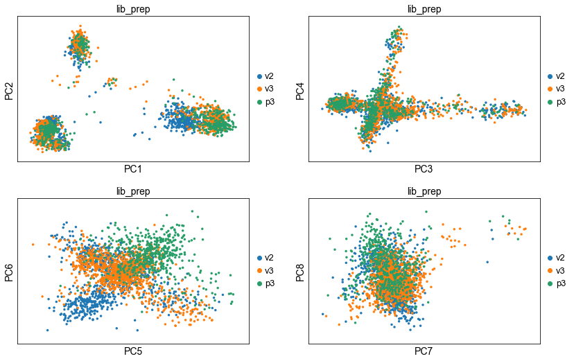
sc.tl.pca(corr_data, svd_solver = 'arpack', use_highly_variable = False)
sc.pl.pca(corr_data, components = ['1,2','3,4','5,6','7,8'], ncols=2, color='lib_prep')
# tSNE
sc.tl.tsne(corr_data, n_pcs = 50)
# UMAP, first with neighbor calculation
sc.pp.neighbors(corr_data, n_pcs = 50, n_neighbors = 20)
sc.tl.umap(corr_data)
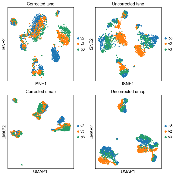
We can now plot the un-integrated and the integrated space reduced dimensions.
fig, axs = plt.subplots(2, 2, figsize=(8,8),constrained_layout=True)
sc.pl.tsne(corr_data, color="lib_prep", title="Corrected tsne", ax=axs[0,0], show=False)
sc.pl.tsne(adata, color="lib_prep", title="Uncorrected tsne", ax=axs[0,1], show=False)
sc.pl.umap(corr_data, color="lib_prep", title="Corrected umap", ax=axs[1,0], show=False)
sc.pl.umap(adata, color="lib_prep", title="Uncorrected umap", ax=axs[1,1], show=False)
Finally, lets save the integrated data for further analysis.
save_file = './data/scanpy_mnn_corrected_3pbmc.h5ad'
corr_data.write_h5ad(save_file)
# create a new object with raw counts
adata_combat = sc.AnnData(X=adata.raw.X, var=adata.raw.var, obs = adata.obs)

#normalize and log-transform
sc.pp.normalize_per_cell(adata_combat, counts_per_cell_after=1e4)
sc.pp.log1p(adata_combat)

# first store the raw data
adata_combat.raw = adata_combat

# run combat
sc.pp.combat(adata_combat, key='lib_prep')
sc.pp.highly_variable_genes(adata_combat)
print("Highly variable genes: %d"%sum(adata_combat.var.highly_variable))
sc.pl.highly_variable_genes(adata_combat)


sc.pp.pca(adata_combat, n_comps=30, use_highly_variable=True, svd_solver='arpack')

sc.pp.neighbors(adata_combat, n_pcs =30)

sc.tl.umap(adata_combat)
sc.tl.tsne(adata_combat, n_pcs = 30)

# compare var_genes
var_genes_combat = adata_combat.var.highly_variable
print("With all data %d"%sum(var_genes_all))
print("With combat %d"%sum(var_genes_combat))
print("Overlap %d"%sum(var_genes_all & var_genes_combat))

print("With 2 batches %d"%sum(var_select))
print("Overlap %d"%sum(var_genes_combat & var_select))
fig, axs = plt.subplots(2, 2, figsize=(8,8),constrained_layout=True)
sc.pl.tsne(corr_data, color="lib_prep", title="MNN tsne", ax=axs[0,0], show=False)
sc.pl.tsne(adata_combat, color="lib_prep", title="Combat tsne", ax=axs[0,1], show=False)
sc.pl.umap(corr_data, color="lib_prep", title="MNN umap", ax=axs[1,0], show=False)
sc.pl.umap(adata_combat, color="lib_prep", title="Combat umap", ax=axs[1,1], show=False)

Scanorama
Try out Scanorama for data integration as well.
To run Scanorama, you need to install python-annoy (already included in conda environment) and scanorama with pip.
We can run scanorama to get a corrected matrix with the correct function, or to just get the data projected onto a new common dimension with the function integrate. For now, run with just integration.
import scanorama


#subset the individual dataset to the same variable genes as in MNN-correct.
alldata2 = dict()
for ds in alldata.keys():
    print(ds)
    alldata2[ds] = alldata[ds][:,var_genes]

#convert to list of AnnData objects
adatas = list(alldata2.values())

# run scanorama.integrate
scanorama  = scanorama.integrate_scanpy(adatas, dimred = 50,)
# returns a list of 3 np.ndarrays with 50 columns.

print(scanorama[0].shape)
print(scanorama[1].shape)
print(scanorama[2].shape)

# make inteo one matrix.
all_s = np.concatenate(scanorama)
print(all_s.shape)

# add to the AnnData object
adata.obsm["SC"] = all_s
# tsne and umap
sc.pp.neighbors(adata, n_pcs =50, use_rep = "SC")
sc.tl.umap(adata)
sc.tl.tsne(adata, n_pcs = 50, use_rep = "SC")
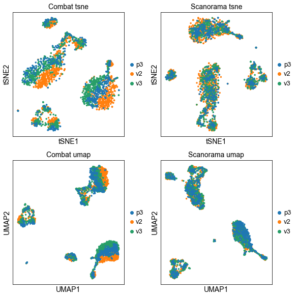
fig, axs = plt.subplots(2, 2, figsize=(8,8),constrained_layout=True)
sc.pl.tsne(adata_combat, color="lib_prep", title="Combat tsne", ax=axs[0,0], show=False)
sc.pl.tsne(adata, color="lib_prep", title="Scanorama tsne", ax=axs[0,1], show=False)
sc.pl.umap(adata_combat, color="lib_prep", title="Combat umap", ax=axs[1,0], show=False)
sc.pl.umap(adata, color="lib_prep", title="Scanorama umap", ax=axs[1,1], show=False)