Example of scater package for QC
Author: Åsa Björklund
Detailed tutorial of scater package at: https://www.bioconductor.org/packages/release/bioc/vignettes/scater/inst/doc/vignette-qc.html
We recommend that you follow steps 1-3 in the tutorial.
Many other packages builds on the SingleCellExperiment class in scater, so it is important that you learn properly how to create an SCE from your data and understand the basics of the scater package.
For this exercise you can either run with your own data or with the example data that they provide with the package. Below is an example with human innate lympoid cells (ILCs) from Bjorklund et al. 2016.
If you want to run the package with the ILCs, all data is available in the course uppmax folder with subfolder: scrnaseq_course/data/ILC/
OBS! As of July 2017, scater has switched from the SCESet class previously defined within the package to the more widely applicable SingleCellExperiment class. From Bioconductor 3.6 (October 2017), the release version of scater will use SingleCellExperiment.
Load packages
suppressMessages(library(scater))
Read data and create a scater SCESet
# read in meta data table and create pheno data
M <- read.table("data/ILC/Metadata_ILC.csv", sep=",",header=T)

# read rpkm values and counts
R <- read.table("data/ILC/ensembl_rpkmvalues_ILC.csv",sep=",",header=T)
C <- read.table("data/ILC/ensembl_countvalues_ILC.csv",sep=",",header=T)
Create the SCESet
# create an SCESet
example_sce <- SingleCellExperiment(assays = list(counts = as.matrix(C)), colData = M)

# you can also add in expression values from the rpkm matrix
# instead of using logged counts.
exprs(example_sce) <- log2(as.matrix(R)+1)
assay(example_sce, "exprs") <- exprs(example_sce)

# you can access the rpkm or count matrix with the commands "counts" and "exprs"
counts(example_sce)[10:13,1:5]
##                 T74_P1_A9_ILC1 T74_P1_B4_NK T74_P1_B7_ILC2 T74_P1_B9_NK
## ENSG00000001167              0            0              0            0
## ENSG00000001460              0            0              0            0
## ENSG00000001461              0         1035              1            1
## ENSG00000001497              0            0              0            0
##                 T74_P1_D10_ILC2
## ENSG00000001167               0
## ENSG00000001460               0
## ENSG00000001461               2
## ENSG00000001497               0
exprs(example_sce)[10:13,1:5]
##                 T74_P1_A9_ILC1 T74_P1_B4_NK T74_P1_B7_ILC2 T74_P1_B9_NK
## ENSG00000001167              0     0.000000      0.0000000    0.0000000
## ENSG00000001460              0     0.000000      0.0000000    0.0000000
## ENSG00000001461              0     6.615791      0.2243554    0.2142426
## ENSG00000001497              0     0.000000      0.0000000    0.0000000
##                 T74_P1_D10_ILC2
## ENSG00000001167       0.0000000
## ENSG00000001460       0.0000000
## ENSG00000001461       0.8229705
## ENSG00000001497       0.0000000
We have accessor functions to access elements of the SingleCellExperiment object.
- counts(object): returns the matrix of read counts. As you can see above, if no counts are defined for the object, then the counts matrix slot is simpy NULL.
- exprs(object): returns the matrix of (log-counts) expression values, in fact accessing the logcounts slot of the object (synonym for logcounts).
For convenience (and backwards compatibility with SCESet) getters and setters are provided as follows: exprs, tpm, cpm, fpkm and versions of these with the prefix “norm_”)
The closest to rpkms is in this case fpkms, so we use fpkm.
It also has slots for:
- Cell metadata, which can be supplied as a DataFrame object, where rows are cells, and columns are cell attributes (such as cell type, culture condition, day captured, etc.).
- Feature metadata, which can be supplied as a DataFrame object, where rows are features (e.g. genes), and columns are feature attributes, such as Ensembl ID, biotype, gc content, etc.
QC stats
Use scater package to calculate qc-metrics
# first check which genes are spike-ins if you have included those
ercc <- grep("ERCC_",rownames(R))

# specify the ercc as feature control genes and calculate all qc-metrics
example_sce <- calculateQCMetrics(example_sce,
                                  feature_controls = list(ERCC = ercc))

# check what all entries are -
colnames(colData(example_sce))
##  [1] "Samples"
##  [2] "Plate"
##  [3] "Donor"
##  [4] "Celltype"
##  [5] "total_features"
##  [6] "log10_total_features"
##  [7] "total_counts"
##  [8] "log10_total_counts"
##  [9] "pct_counts_top_50_features"
## [10] "pct_counts_top_100_features"
## [11] "pct_counts_top_200_features"
## [12] "pct_counts_top_500_features"
## [13] "total_features_endogenous"
## [14] "log10_total_features_endogenous"
## [15] "total_counts_endogenous"
## [16] "log10_total_counts_endogenous"
## [17] "pct_counts_endogenous"
## [18] "pct_counts_top_50_features_endogenous"
## [19] "pct_counts_top_100_features_endogenous"
## [20] "pct_counts_top_200_features_endogenous"
## [21] "pct_counts_top_500_features_endogenous"
## [22] "total_features_feature_control"
## [23] "log10_total_features_feature_control"
## [24] "total_counts_feature_control"
## [25] "log10_total_counts_feature_control"
## [26] "pct_counts_feature_control"
## [27] "pct_counts_top_50_features_feature_control"
## [28] "total_features_ERCC"
## [29] "log10_total_features_ERCC"
## [30] "total_counts_ERCC"
## [31] "log10_total_counts_ERCC"
## [32] "pct_counts_ERCC"
## [33] "pct_counts_top_50_features_ERCC"
## [34] "is_cell_control"
A more detailed description can be found at the tutorial site, or by running: ?calculateQCMetrics
If you have additional qc-metrics that you want to include, like mapping stats, rseqc data etc, you can include all of that in your phenoData.
Look at data interactively in GUI
You can play around with the data interactively with the shiny app they provide. OBS! It takes a while to load and plot, so be patient.
# you can open the interactive gui with:
scater_gui(example_sce)
Plots of expression values
Different ways of visualizing gene expression per batch/celltype etc.
# plot detected genes at different library depth for different plates and celltypes
plotScater(example_sce, block1 = "Plate", block2 = "Celltype",
     colour_by = "Celltype", nfeatures = 300, exprs_values = "exprs")

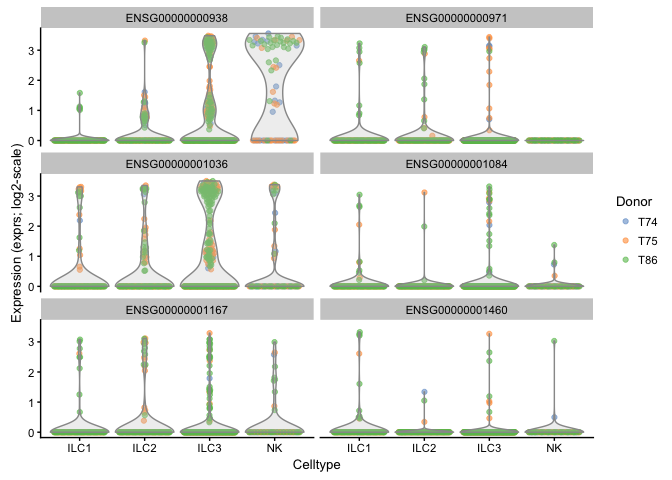
# violin plot for gene expression
plotExpression(example_sce, rownames(example_sce)[6:11],
               x = "Celltype", exprs_values = "exprs",
               colour = "Donor",log=TRUE)
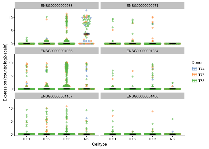
plotExpression(example_sce, rownames(example_sce)[6:11],
               x = "Celltype", exprs_values = "counts", colour = "Donor",
               show_median = TRUE, show_violin = FALSE,  log = TRUE)
You can play around with all the arguments in plotExpression, for example:
- log=TRUE/FALSE
- show_violin=TRUE/FALSE
- show_median=TRUE/FALSE
- exprs_values=”counts”/”exprs”
And specify different coloring and and batches to plot by that are defined in the CellMetadata (ex-phenoData in the SCESet class).
QC overview and filtering
There are several ways to plot the QC summaries of the cells in the scater package. A few examples are provided below. In this case, cells have already been filtered to remove low quality samples, so no filtering step is performed.
# first remove all features with no/low expression, here set to expression in more than 5 cells with > 1 count
keep_feature <- rowSums(counts(example_sce) > 1) > 5
example_sce <- example_sce[keep_feature,]
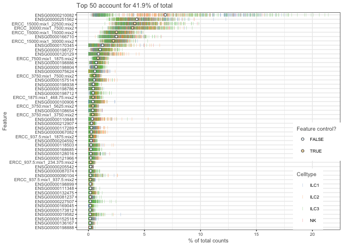
## Plot highest expressed genes.
plotQC(example_sce, type = "highest-expression",col_by="Celltype")
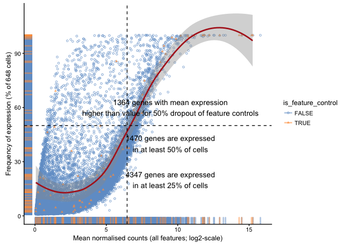
Plot frequency of expression (number of cells with detection) vs mean normalised expression.
plotExprsFreqVsMean(example_sce)
## `geom_smooth()` using method = 'loess'
Plot log10 total count vs number of cells a gene is detected in.
plotFeatureData(example_sce, aesth = aes_string(x = "n_cells_counts", y =
"log10_total_counts"))

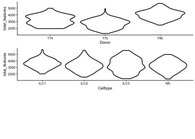
Plot different qc-metrics per batch.
p1 <- plotPhenoData(example_sce, aes(x = Donor, y = total_features,
                                    colour = log10_total_counts))

p2 <- plotPhenoData(example_sce, aes(x = Celltype, y = total_features,
                                     colour = log10_total_counts))

multiplot(p1, p2, rows = 2)
## [1] 2
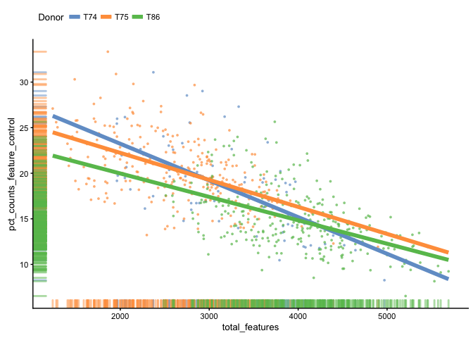
Plot the percentage of expression accounted for by feature controls against total_features.
plotPhenoData(example_sce,
      aes(x = total_features, y = pct_counts_feature_control, colour = Donor)) +
      theme(legend.position = "top") +
      stat_smooth(method = "lm", se = FALSE, size = 2, fullrange = TRUE)
Dimensionality reduction plots
Plot the cells in reduced space and define color/shape/size by different qc-metrics or meta-data entries.
# PCA - with different coloring, first 4 components
# first by Donor
plotPCA(example_sce,ncomponents=4,colour_by="Celltype",shape_by="Donor")
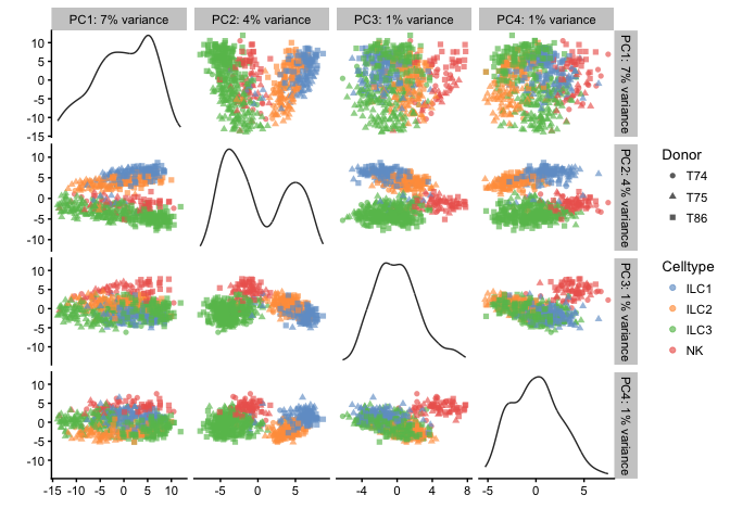
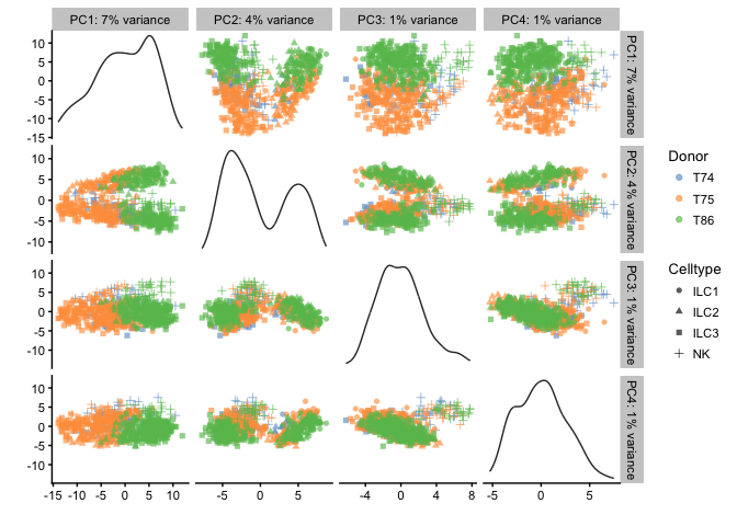
# then by Celltype
plotPCA(example_sce,ncomponents=4,colour_by="Donor",shape_by="Celltype")
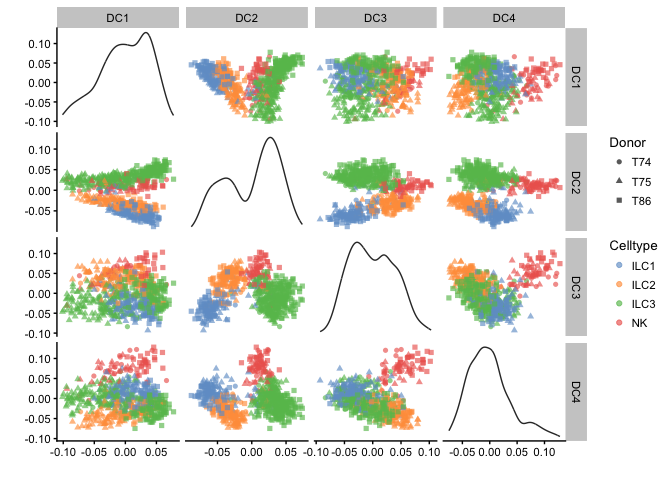
# Diffusion map
plotDiffusionMap(example_sce, colour_by="Celltype",shape_by="Donor",ncomponents=4)
# tSNE - uses Rtsne function to run tsne
plotTSNE(example_sce, colour_by="Celltype",shape_by="Donor", ntop=30, perplexity=30 )

For all of these dimensionality reduction methods, you can specify return_SCE = TRUE and it will return an SCESet object with the slot reducedDimension filled. This can be usefule if PCA/tSNE takes long time to run and you want to plot several different colors etc.
You can later plot the reduced dimension with plotReducedDim.
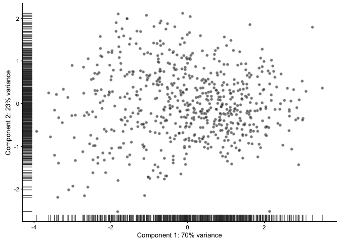
PCA based on QC-measures
PCA based on the phenoData can be used to detect outlier cells with qc-measures that deviates from the rest. But be careful with checking how these cells deviate before taking a decision on why to remove them.
OBS! detection of outlier requires that package mvoutlier is installed.
example_sce <- plotPCA(example_sce, pca_data_input = "pdata",
                          detect_outliers = TRUE, return_SCE = TRUE)
## The following selected_variables were not found in colData(object): pct_counts_feature_controlsThe following selected_variables were not found in colData(object): total_features_feature_controlsThe following selected_variables were not found in colData(object): log10_total_counts_feature_controls

## Other variables from colData(object) can be used by specifying a vector of variable names as the selected_variables argument.

## PCA is being conducted using the following variables:pct_counts_top_100_featurestotal_featureslog10_total_counts_endogenous

## sROC 0.1-2 loaded
# we can use the filter function to remove all outlier cells
filtered_sce <- filter(example_sce, outlier==FALSE)
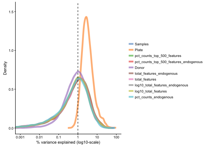
QC of experimental variables
Median marginal R2 for each variable in pData(example_sceset) when fitting a linear model regressing exprs values against just that variable. Shows how much of the data variation is explained by a single variable.
plotQC(example_sce, type = "expl")
## The variable pct_counts_top_50_features_feature_control only has one unique value, so R^2 is not meaningful.
## This variable will not be plotted.

## The variable pct_counts_top_50_features_ERCC only has one unique value, so R^2 is not meaningful.
## This variable will not be plotted.

## The variable is_cell_control only has one unique value, so R^2 is not meaningful.
## This variable will not be plotted.

## The variable outlier only has one unique value, so R^2 is not meaningful.
## This variable will not be plotted.
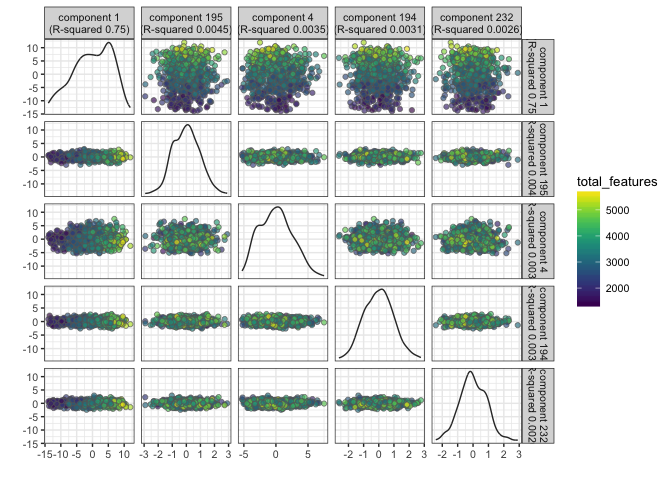
Identify PCs that correlate strongly to certain QC or Meta-data values
# for total_features
plotQC(example_sce, type = "find-pcs", variable = "total_features", plot_type = "pairs-pcs")
# for Donor
plotQC(example_sce, type = "find-pcs", variable = "Donor", plot_type = "pairs-pcs")

PC1 clearly correlates to total_features, which is a common problem in scRNAseq data. This may be a technical artifact, or a biological features of celltypes with very different sizes.
It is also clear that PC1 separates out the different donors.
Session info
sessionInfo()
## R version 3.4.1 (2017-06-30)
## Platform: x86_64-apple-darwin15.6.0 (64-bit)
## Running under: macOS Sierra 10.12.6
##
## Matrix products: default
## BLAS: /Library/Frameworks/R.framework/Versions/3.4/Resources/lib/libRblas.0.dylib
## LAPACK: /Library/Frameworks/R.framework/Versions/3.4/Resources/lib/libRlapack.dylib
##
## locale:
## [1] en_US.UTF-8/en_US.UTF-8/en_US.UTF-8/C/en_US.UTF-8/en_US.UTF-8
##
## attached base packages:
## [1] stats4    parallel  stats     graphics  grDevices utils     datasets
## [8] methods   base
##
## other attached packages:
##  [1] bindrcpp_0.2               scater_1.6.2
##  [3] SingleCellExperiment_1.0.0 SummarizedExperiment_1.8.1
##  [5] DelayedArray_0.4.1         matrixStats_0.53.0
##  [7] GenomicRanges_1.30.1       GenomeInfoDb_1.14.0
##  [9] IRanges_2.12.0             S4Vectors_0.16.0
## [11] ggplot2_2.2.1              Biobase_2.38.0
## [13] BiocGenerics_0.24.0
##
## loaded via a namespace (and not attached):
##   [1] backports_1.1.2        Hmisc_4.1-1            RcppEigen_0.3.3.3.1
##   [4] plyr_1.8.4             igraph_1.1.2           lazyeval_0.2.1
##   [7] sp_1.2-7               shinydashboard_0.6.1   splines_3.4.1
##  [10] digest_0.6.15          htmltools_0.3.6        viridis_0.5.0
##  [13] magrittr_1.5           checkmate_1.8.5        memoise_1.1.0
##  [16] cluster_2.0.6          limma_3.34.8           xts_0.10-1
##  [19] prettyunits_1.0.2      colorspace_1.3-2       blob_1.1.0
##  [22] rrcov_1.4-3            dplyr_0.7.4            RCurl_1.95-4.10
##  [25] tximport_1.6.0         lme4_1.1-15            bindr_0.1
##  [28] survival_2.41-3        zoo_1.8-1              glue_1.2.0
##  [31] gtable_0.2.0           zlibbioc_1.24.0        XVector_0.18.0
##  [34] MatrixModels_0.4-1     kernlab_0.9-25         car_2.1-6
##  [37] prabclus_2.2-6         DEoptimR_1.0-8         SparseM_1.77
##  [40] VIM_4.7.0              scales_0.5.0           sgeostat_1.0-27
##  [43] mvtnorm_1.0-7          GGally_1.3.2           DBI_0.7
##  [46] edgeR_3.20.8           sROC_0.1-2             Rcpp_0.12.15
##  [49] viridisLite_0.3.0      xtable_1.8-2           progress_1.1.2
##  [52] laeken_0.4.6           htmlTable_1.11.2       foreign_0.8-69
##  [55] bit_1.1-12             proxy_0.4-21           mclust_5.4
##  [58] Formula_1.2-2          vcd_1.4-4              htmlwidgets_1.0
##  [61] httr_1.3.1             fpc_2.1-11             RColorBrewer_1.1-2
##  [64] modeltools_0.2-21      acepack_1.4.1          flexmix_2.3-14
##  [67] reshape_0.8.7          pkgconfig_2.0.1        XML_3.98-1.9
##  [70] nnet_7.3-12            locfit_1.5-9.1         labeling_0.3
##  [73] rlang_0.1.6            reshape2_1.4.3         AnnotationDbi_1.40.0
##  [76] munsell_0.4.3          tools_3.4.1            RSQLite_2.0
##  [79] pls_2.6-0              cvTools_0.3.2          evaluate_0.10.1
##  [82] stringr_1.2.0          yaml_2.1.16            knitr_1.19
##  [85] bit64_0.9-7            robustbase_0.92-8      nlme_3.1-131
##  [88] mime_0.5               quantreg_5.34          biomaRt_2.34.2
##  [91] compiler_3.4.1         pbkrtest_0.4-7         rstudioapi_0.7
##  [94] beeswarm_0.2.3         curl_3.1               e1071_1.6-8
##  [97] smoother_1.1           tibble_1.4.2           robCompositions_2.0.6
## [100] pcaPP_1.9-73           stringi_1.1.6          trimcluster_0.1-2
## [103] lattice_0.20-35        Matrix_1.2-12          nloptr_1.0.4
## [106] pillar_1.1.0           lmtest_0.9-35          data.table_1.10.4-3
## [109] cowplot_0.9.2          bitops_1.0-6           httpuv_1.3.5
## [112] R6_2.2.2               latticeExtra_0.6-28    gridExtra_2.3
## [115] vipor_0.4.5            boot_1.3-20            MASS_7.3-48
## [118] assertthat_0.2.0       destiny_2.6.1          rhdf5_2.22.0
## [121] rprojroot_1.3-2        rjson_0.2.15           GenomeInfoDbData_1.0.0
## [124] diptest_0.75-7         mgcv_1.8-23            grid_3.4.1
## [127] rpart_4.1-12           class_7.3-14           minqa_1.2.4
## [130] rmarkdown_1.8          mvoutlier_2.0.8        Rtsne_0.13
## [133] TTR_0.23-3             shiny_1.0.5            base64enc_0.1-3
## [136] ggbeeswarm_0.6.0