ChIP-seq with exogenous chromatin spike
Requirements
-
R 3.5.0 (2018-04-23) or newer
-
Bioconductor packages:
- ChIPSeqSpike
- BSgenome.Hsapiens.UCSC.hg38
Data
We will use ChIP-seq of H3K79me2 from Orlando et al, 2014 (“Quantitative ChIP-Seq Normalization Reveals Global Modulation of the Epigenome”).
The histone H3 lysine-79 dimethyl (H3K79me2) modification is catalyzed by the DOT1L protein and is associated with the release of paused RNA Polymerase II and licensing of transcriptional elongation. This modification is typically deposited within the 5′ regions of genes.
The experimental design was as follows:
- Jurkat cells were treated with selective DOT1L inhibitor EPZ5676 to globally deplete H3K79me2;
- chromatin from treated and untreated cells was mixed in different proportions (here we use two conditions: 100 % treated and 50-50% treated + untreated) to mimic a global change in abundance of H3K79me2
- chromatin from Drosophila S2 cells was added in a 1:2 ratio (1 S2 cell per 2 Jurkat cells) which provided a constant “reference” amount of H3K79me2 per human cell.
GEO accession is GSE60104
ENA accession is ` PRJNA257491`
files in the dataset:
| sample | GEO accession | SRA accession |
|---|---|---|
| Jurkat_K79_100%_R1 | GSM1465008 | SRR1536561 |
| Jurkat_K79_100%_R2 | GSM1464998 | SRR1536551 |
| Jurkat_K79_50%_R1 | GSM1465006 | SRR1536559 |
| Jurkat_WCE_100%_R1 | GSM1511469 | SRR1584493 |
| Jurkat_WCE_100%_R2 | GSM1511474 | SRR1584498 |
| Jurkat_WCE_50%_R1 | GSM1511467 | SRR1584491 |
Data preparation
All data processing steps were already performed.
Raw fastq reads were filtered so that low quality bases and adapters were removed. Reads were mapped to the composite reference which consisted of hg38 and dm6 using bowtie. Only reads with one best alignemnt were retained. Alignments were split by reference using samtools and were subset to chromosome 1 for hg38 and chromosome 2L for dm6.
Quality metrics were computed for each bam split by reference genome.
Fixed-step bigWig files were generated as follows:
-
genome coverage of data in
bamfiles at 1 bp resolution was calculated usingbedtools -
covareage was converted to fixed step
wigfiles using https://gist.github.com/svigneau/8846527/bedgraph_to_wig.pl using step size 100 -
wigwas converted tobigWigusing UCSC toolkit using chrom.sizes forhg38downloaded from UCSC genome browser
bedtools genomecov -bga -ibam in.bam >out.bg

bedgraph_to_wig.pl --bedgraph out.bg --wig out.wig --step 100

wigToBigWig out.wig chrom.sizes final.bw
All files necessary to execute the code in R can be copied from Rackham from:
/sw/share/compstore/courses/ngsintro/chipseq/exospike/exospike.tar.gz
After copying the files please decompress the archive and note the path to folder /chip_exo_spike on your local system.
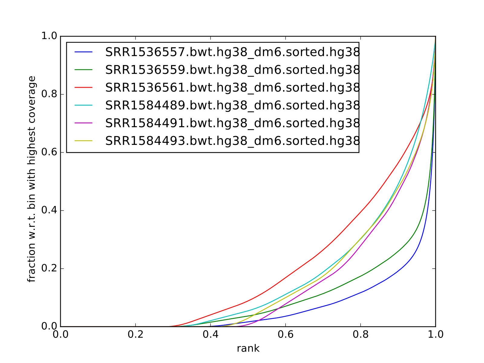
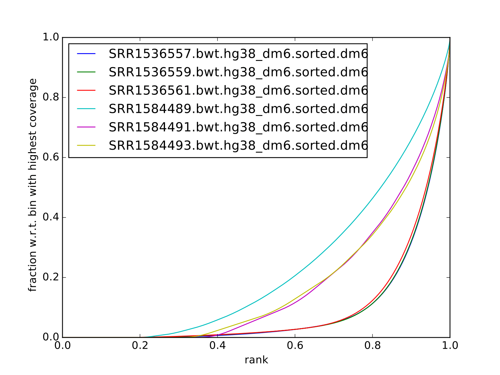
Fingerprint plots
all reads mapped to hg38 (i.e. not subset):
all reads mapped to dm6 (i.e. not subset):
Disclaimer
Please be aware that this is an experimental code, and as such does not represent any golden standard for analyses of this type. This is my exploration of the topic of using exogenous chromatic spike for ChIP-seq. I will aim to keep updating it with further steps of the analysis, once I get there.
Using ChIPSeqSpike for ChIPseq signal scaling
This workflow is based on https://github.com/descostesn/BiocNYC-ChIPSeqSpike.
The scaling procedure works on computers with non-Windows operating systems. This includes Uppmax, so you can use salloc command to book a node and follow the workflow remotely.
Files and directories
In R:
workdir="/path/to/chip_exo_spike"
setwd(workdir)

bam_path=file.path(workdir,"bam")
bw_path=file.path(workdir,"tracks")
exp_data=file.path(workdir,"exp_data.csv")

#you will have to copy the initial bigwig tracks to the output folder at a later stage
#output_folder=file.path(workdir,"results")
#dir.create(output_folder)

#so until the package code is fixed:
output_folder=bw_path
You can inspect the file exp_data.csv to familiarize yourself with the structure:
info=read.table(exp_data, sep=",")
head(info)
Scaling of signal to exogenous chromatin spike
Load the library and create the object:
library(ChIPSeqSpike)

cs <- spikeDataset(exp_data, bam_path, bw_path)
Calculate the size factors based on numbers of mapped reads:
cs <- estimateScalingFactors(cs, verbose = TRUE)
> spikeSummary(cs)
                endoScalFact exoScalFact endoCount exoCount
H3K79me2_0         0.5367522   1.0216143   1863057   978843
input              1.1604563          NA    861730       NA
H3K79me2_50        0.6604427   0.7663511   1514136  1304885
input              2.9039209          NA    344362       NA
H3K79me2_100_r1    1.5994012   0.3687641    625234  2711761
input              2.5008003          NA    399872       NA
H3K79me2_100_r2    2.6171433   0.6153835    382096  1625003
input              7.7456934          NA    129104       NA
RPM scaling. The first normalization applied to the data is the ‘Reads Per Million’ (RPM) mapped reads. The method ‘scaling’ is used to achieve this normalization using default parameters.
cs <- scaling(cs, outputFolder = output_folder)
You are supposed to obtain files *-RPM.bw after this step.
Input subtraction. This step is to subtract background (from input samples) from signal. The inputSubtraction method simply subtracts scores of the input DNA experiment from the corresponding ones.
cs <- inputSubtraction(cs)
You are supposed to obtain *-RPM-BGSub.bw after this step.
RPM scaling reversal. After RPM and input subtraction normalization, the RPM normalization is reversed in order for the data to be normalized by the exogenous scaling factors.
cs<- scaling(cs, reverse = TRUE)
*-RPM-BGSub-reverted.bw files after this step.
Exogenous Scaling. Finally, exogenous scaling factors are applied to the data.
cs <- scaling(cs, type = "exo")
The end result: *-RPM-BGSub-reverted-spiked.bw files after this step.
Extracting binding values. The last step of data processing is to extract and format binding scores in order to use plotting methods. The extractBinding method extracts binding scores at different locations and stores these values in the form of PlotSetArray objects and matrices. The scores are retrieved on annotations provided in a gff file. If one wishes to focus on peaks, their coordinates should be submitted at this step. The genome name must also be provided. For details about installing the required BSgenome package corresponding to the endogenous organism, see the BSgenome package documentation.
Please note that this steps may take a long time.
gff=file.path(workdir,"hg38_refseq_chr1.gtf")
library(BSgenome.Hsapiens.UCSC.hg38)

cs <- extractBinding(cs, gff_vec=gff, genome="hg38")
After this step, save the workspace
save.image(file = "chipseqspike.RData")
To load the data:
load("chipseqspike.RData")
Data visualization.
ChIPSeqSpike offers several graphical methods for normalization diagnosis and data exploration. These choices enable one to visualize each step of the normalization through exploring intersamples differences using profiles, heatmaps, boxplots and correlation plots.
When performing this exercise on Uppmax, save the plots to pdf for viewing:
pdf("filename.pdf")
## here command to produce the plot
dev.off()
Visualization with gene meta-profiles
The first step of spike-in normalized ChIP-Seq data analysis is an inter-sample comparison by meta-gene or meta-annotation profiling. The method plotProfile automatically plots all experiments at the start, midpoint, end and composite locations of the annotations provided to the method extractBinding in gff format. The effect of each transformation on a particular experiment can be visualized with plotTransform.
## Plot spiked-in data
plotProfile(cs, legends = TRUE)

## Add profiles before transformation
plotProfile(cs, legends = TRUE, notScaled=TRUE)

## Visualize the effect of each transformation on each experiment
plotTransform(cs, legends = TRUE, separateWindows = TRUE)
Visualization with Boxplots
boxplotSpike plots boxplots of the mean values of ChIP-seq experiments on the annotations given to the extractBinding method.
## Boxplot of the spiked-in data
boxplotSpike(cs, outline = FALSE)

## Boxplot of the raw data
boxplotSpike(cs,rawFile = TRUE, spiked = FALSE, outline=FALSE)

## Boxplot of all transformations
boxplotSpike(cs,rawFile = TRUE, rpmFile = TRUE, bgsubFile = TRUE, revFile = TRUE, spiked = TRUE, outline = FALSE)
Correlation plots
The plotCor method plots the correlation between ChIP-seq experiments using heatscatter plot.
## Log transform correlation plot of spiked data with heatscatter representation
plotCor(cs, rawFile = FALSE, rpmFile = FALSE,  bgsubFile = FALSE,  revFile = FALSE, spiked = TRUE,  main = "heatscatter",  method_cor = "spearman", add_contour = FALSE,  nlevels = 10,  color_contour = "black", method_scale = "log",  allOnPanel = TRUE, separateWindows = FALSE,  verbose = FALSE)

## Plot as above with raw data
plotCor(cs, rawFile = TRUE, rpmFile = FALSE,  bgsubFile = FALSE,  revFile = FALSE, spiked = FALSE,  main = "heatscatter",  method_cor = "spearman", add_contour = FALSE,  nlevels = 10,  color_contour = "black", method_scale = "log",  allOnPanel = TRUE, separateWindows = FALSE,  verbose = FALSE)

## Correlation table comparing all transformations
corr_matrix <- plotCor(cs, rawFile = TRUE, rpmFile = TRUE, bgsubFile = TRUE, revFile = TRUE, spiked = TRUE, heatscatterplot = FALSE, verbose = TRUE)
What to do next
- use scaled
bigWigtracks to view the signal in IGV - use
bedfiles produced from scaledbigWigsto perform peak calling for instance with MACS2 - differential binding analysis using
csaw(more appropriate for broad marks) inputing the scaling factors obtained from scaling byChIPSeqSpike - perform the normalisation / scaling directly in
csaw - use scaled
bed/bigwigfor data exploration using PCA and MA plots