Detection of broad peaks from ChIP-seq data
Requirements
- MACS 2.1.2 (this version is not available as a module on Rackham)
- R 3.5.0 (2018-04-23) or newer
- csaw and its dependencies
Bioconductor packages required for annotation:
- org.Hs.eg.db
- TxDb.Hsapiens.UCSC.hg38.knownGene
Please note that this lab consists of two parts: (i) calling broad peaks using MACS (on Uppmax) and (ii) finding enriched genomic windows using R and csaw (local).
MACS 2.1.2 installation (on Uppmax):
in your home folder on Rackham:
## clone pyenv repository from github
git clone git://github.com/yyuu/pyenv.git ~/.pyenv

## make pyenv start at a login
echo 'export PYENV_ROOT="$HOME/.pyenv"' >> ~/.bash_profile
echo 'export PATH="$PYENV_ROOT/bin:$PATH"' >> ~/.bash_profile
echo 'eval "$(pyenv init -)"' >> ~/.bash_profile

source ~/.bash_profile

## install required version of python and set it to use
pyenv install 2.7.9
pyenv global 2.7.9

## create directory for macs2
mkdir macs2
cd macs2

## clone macs repository from github
git clone https://github.com/taoliu/MACS.git

## install MACS2 with its dependencies
pip install MACS2

## export the location of /macs/MACS/bin folder to $PATH
## to obtain the path you can use `pwd`

in my case:
export PATH=$PATH:/home/agata/soft/macs/MACS/bin
The detailed instructions on how to install and use pyenv on Uppmax are at
https://www.uppmax.uu.se/support/user-guides/python-modules-guide/
Instructions how to install R and Bioconductor packages (including dependencies for csaw) can be found in instructions to previous labs. Please note that this workflow has been tested using R 3.5.0 and csaw 1.14.1.
Data
We will use ChIP-seq of H3K79me2 from Orlando et al, 2014 (“Quantitative ChIP-Seq Normalization Reveals Global Modulation of the Epigenome”). H3K79me2 is enriched at active promoters and linked to transcriptional activation. This is a SE data set, which admitedly is not the best design for broad marks. To use this procedure with PE data, please follow modifications listed on https://github.com/taoliu/MACS.
GEO accession is GSE60104
ENA accession is ` PRJNA257491`
files in the dataset:
| sample | GEO accession | SRA accession |
|---|---|---|
| Jurkat_K79_100%_R1 | GSM1465008 | SRR1536561 |
| Jurkat_K79_100%_R2 | GSM1464998 | SRR1536551 |
| Jurkat_K79_50%_R1 | GSM1465006 | SRR1536559 |
| Jurkat_K79_0%_R1 | GSM1465004 | SRR1536557 |
| Jurkat_WCE_100%_R1 | GSM1511469 | SRR1584493 |
| Jurkat_WCE_100%_R2 | GSM1511474 | SRR1584498 |
| Jurkat_WCE_50%_R1 | GSM1511467 | SRR1584491 |
| Jurkat_WCE_0%_R1 | GSM1511465 | SRR1584489 |
We will call peaks from one sample only, and compare the results to other samples processed earlier.
Data have been processed in the same way as for the TF ChIP-seq, i.e. the duplicated reads were removed, as were the reads mapped to blacklisted regions. In this case the reads were mapped to hg38 assembly of human genome.
Quality control
As always, one should start the analysis from assesment of data quality. This is already performed, and the plots and metrics are below.
Cross-correlation and related metrics
The files discussed in this section can be accessed at
/sw/share/compstore/courses/ngsintro/chipseq/broad_peaks/results_pre/fingerprint
and
/sw/share/compstore/courses/ngsintro/chipseq/broad_peaks/results_pre/xcor
.
These metrics have been developed with application to TF ChIP-seq in mind, and you can see that the results for broad peaks are not as easy to interpret as for point-source factors. Below are cross correlation plots for the IP and input you are going to use for the exercise. Already from these plots alone it is evident that the data has some quality issues. At this point you should be able to identify them.
ChIP:

input:
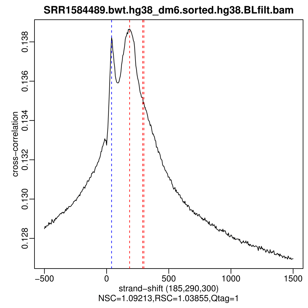
As for the ChIP, the cross correlation profile of factors with broad occupancy patterns is not going to be as sharp as for TFs, and the values of NSC and RSC tend to be lower, which does not mean that the ChIP failed. In fact, the developers of the tool do not recommend using the same NSC / RSC values as quality cutoffs for broad marks. However, input samples should not display signs of enrichment, as is the case here.
Cumulative enrichment
Another plot worth examining is cumulative enrichment (aka fingerprint from deepTools):
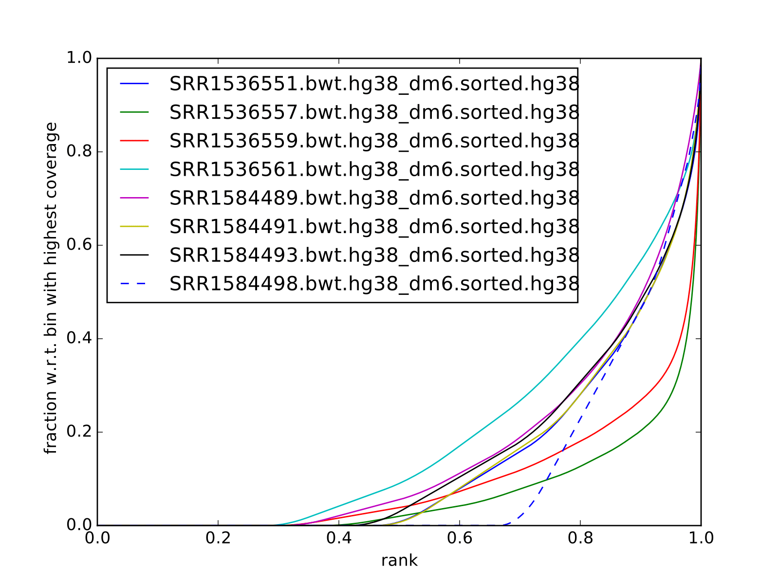
You can see that even though the cross correlation metrics don’t look great, to put it mildly, some enrichment can be observed for the ChIP samples, and not for the input samples. As this data is data from very shallow sequencing, the fraction of the genome covered by reads is smaller than expected (0.3 for the best sample). Thus we do not expect to detect all occupancy sites, only the ones which give the strongest signal (this is actually an advantage for this class, as it reduces the running time).
Peak calling
You will call peaks using sample Jurkat_K79_50_R1 (SRR1536557) and its matching input SRR1584489.
Effective genome size for hg38 is 3.0e9.
The estimated fragment size is 180 bps (phantompeakqualtools).
mkdir -p results/macs
cd results/macs

ln -s /sw/share/compstore/courses/ngsintro/chipseq/broad_peaks/bam/SRR1536557.bwt.hg38_dm6.sorted.hg38.BLfilt.bam
ln -s /sw/share/compstore/courses/ngsintro/chipseq/broad_peaks/bam/SRR1584489.bwt.hg38_dm6.sorted.hg38.BLfilt.bam

#if it is a different session than when installing pyenv and macs2:
pyenv global 2.7.9

macs2 callpeak -t SRR1536557.bwt.hg38_dm6.sorted.hg38.BLfilt.bam -c SRR1584489.bwt.hg38_dm6.sorted.hg38.BLfilt.bam -n 50_R1 --outdir 50_R1 -f BAM --gsize 3.0e9 -q 0.1 --nomodel --extsize 180 --broad --broad-cutoff 0.1
If you would like to compare the results of two different methods of finding broad peaks, repeat this with another data set:
ln -s /sw/share/compstore/courses/ngsintro/chipseq/broad_peaks/bam/SRR1536561.bwt.hg38_dm6.sorted.hg38.BLfilt.bam
ln -s /sw/share/compstore/courses/ngsintro/chipseq/broad_peaks/bam/SRR1584493.bwt.hg38_dm6.sorted.hg38.BLfilt.bam

macs2 callpeak -t SRR1536561.bwt.hg38_dm6.sorted.hg38.BLfilt.bam -c SRR1584493.bwt.hg38_dm6.sorted.hg38.BLfilt.bam -n 100_R1 --outdir 100_R1 -f BAM --gsize 3.0e9 -q 0.1 --nomodel --extsize 180 --broad --broad-cutoff 0.1
You can now inspect the results in the output folder 50_R1. The structure is alike the output for calling narrow peaks. The file *.broadPeak is in BED6+3 format which is similar to narrowPeak file used for point-source factors, except for missing the 10th column for annotating peak summits. Look here (https://github.com/taoliu/MACS) for details.
How many peaks were identified?
[agata@r483 50_R1]$ wc -l *Peak
  46664 50_R1_peaks.broadPeak
This is a preliminary peak list, and in case of broad peaks, it almost always needs some processing or filtering.
NOTE:
You can also copy the results from
/sw/share/compstore/courses/ngsintro/chipseq/broad_peaks/results_pre/macs
Visual inspection of the peaks
You will use IGV for this step, and it is recommended that you run it locally on your own computer. Please load hg38 reference genome.
Required files are:
- SRR1536557.bwt.hg38_dm6.sorted.hg38.BLfilt.bam and bai
- SRR1584489.bwt.hg38_dm6.sorted.hg38.BLfilt.bam and bai
- 50_r1_peaks.broadPeak
You can access the bam and bai files from
/sw/share/compstore/courses/ngsintro/chipseq/broad_peaks/bam/.
You can look at the locations of interest. Some peaks with low FDR (q value) or high fold enrichment may be worth checking out. Or check your favourite gene.
Some ideas:
chr1:230,145,433-230,171,784
chr1:235,283,256-235,296,431
chr1:244,857,626-244,864,213
chr1:45,664,079-45,690,431

chr1:45,664,079-45,690,431
The first two locations visualise peaks longer than 2kb. The third and the fourth are a 4 kb-long peaks with fold erichment over background >15.
An example (two upper tracks are ChIP samples, the bottom track is input; the annotation is refseq genes and peaks called for sample 100_r1):
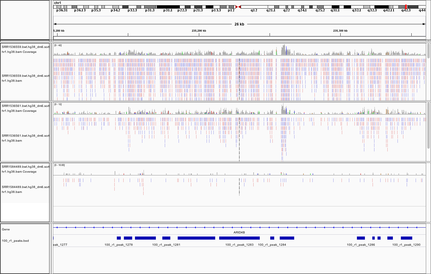
All the above but, perhaps the fifth location most of all, demonstrate one of the common caveats of calling broad peaks: regions obviously enriched in a mark of interest are represented as a series of adjoining peaks which in fact should be merged into one long enrichment domain. You may leave it as is, or merge the peaks into longer ones, depending on the downstream application.
Postprocessing of peak candidates
Please note that this step is only an example, as any postprocessing of peak calling results is highly project specific.
Normally, you would work with replicated data. As in the case of TFs earlier, it is recommended to continue working with peaks reproducible between replicates.
The peak candidate lists can and should be further filtered, based on fold enrichment and pileup value, to remove peaks which could have a high fold enrichment but low signal, as these are likely non-informative. Any filtering, however has to be performed having in mind the biological characteristics of the signal.
You can merge peaks which are close to one another using bedtools (https://bedtools.readthedocs.io/en/latest/). You will control the distance of features to be merged using option -d. Here we arbitrarily choose 1 kb.
cp 50_r1_peaks.broadPeak 50_r1.bed

module load bioinfo-tools
module load BEDTools/2.27.1

bedtools merge -d 1000 -i 50_r1.bed > 50_r1.merged.bed

#how many peaks?
wc -l 50_r1.merged.bed

#11732 50_r1.merged.bed
Alternative approach: window-based enrichment analysis (csaw)
This workflow is similar to the one using csaw designed for TF peaks. The differences pertain to analysis of signal from diffuse marks. Please check the “Csaw (Alternative differential binding analyses)” tutorial for more detailed comments on each step.
You will use data from the same dataset, however, the files were processed in a different manner: the alignments were not filtered to remove duplictae reads nor the reads mapping to the ENCODE blacklisted regions. To reduce the computational burden, the bam files were subset to contain alignments to chr1.
This exercise is best performed locally. It has not been tested on Uppmax.
First, you need to copy the necessary files to your laptop:
cd /desired/location

scp <USERNAME>@rackham.uppmax.uu.se:/sw/share/compstore/courses/ngsintro/chipseq/broad_peaks/broad_peaks_bam.tar.gz .

#type your password at the prompt

tar zcvf broad_peaks_bam.tar.gz
The remaining part of the exercise is performed in R.
Sort out the working directory and file paths:
setwd("/path/to/workdir")

dir.data = "/path/to/desired/location/bam_chr1"

k79_100_1=file.path(dir.data,"SRR1536561.bwt.hg38_dm6.sorted.chr1.hg38.bam")
k79_100_2=file.path(dir.data,"SRR1536561.bwt.hg38_dm6.sorted.chr1.hg38.bam")
k79_100_i1=file.path(dir.data,"SRR1584493.bwt.hg38_dm6.sorted.chr1.hg38.bam")
k79_100_i2=file.path(dir.data,"SRR1584498.bwt.hg38_dm6.sorted.chr1.hg38.bam")

bam.files <- c(k79_100_1,k79_100_2,k79_100_i1,k79_100_i2)
Read in the data:
frag.len=180

library(csaw)

data <- windowCounts(bam.files, ext=frag.len, width=100)
You will identify the enrichment windows by performing a differential occupancy analysis between ChIP and input samples.
Information on the contrast to test:
grouping <- factor(c('chip', 'chip', 'input', 'input'))
design <- model.matrix(~0 + grouping)
colnames(design) <- levels(grouping)
library(edgeR)
contrast <- makeContrasts(chip - input, levels=design)
Next, you need to filter out uninformative windows with low signal prior to further analysis. Selection of appropriate filtering strategy and cutoff is key to a successful detection of differential occupancu events, and is data dependent. Filtering is valid so long as it is independent of the test statistic under the null hypothesis. One possible approach involves choosing a filter threshold based on the fold change over the level of non-specific enrichment (background). The degree of background enrichment is estimated by counting reads into large bins across the genome.
With type="global", the filterWindows function returns the increase in the abundance of
each window over the global background.
Windows are filtered by setting some minimum threshold on this increase. Here, a fold change of 3 is necessary for a window to be considered as containing a binding site.
In this example, you estimate the global background using ChIP samples only. You can do it using the entire dataset of course.
bam.files_chip <- c(k79_100_1,k79_100_2)

bin.size <- 2000L
binned.ip <- windowCounts(bam.files_chip, bin=TRUE, width=bin.size, ext=frag.len)
data.ip=data[,1:2]
filter.stat <- filterWindows(data.ip, background=binned.ip, type="global")

keep <- filter.stat$filter > log2(3)
data.filt <- data[keep,]
To examine how many windows passed the filtering:
summary(keep)

##   Mode   FALSE    TRUE
##  logical   56543   61752
To normalise the data for different library sizes you need to calculate normalisation factors based on large bins:
binned <- windowCounts(bam.files, bin=TRUE, width=10000)
data.filt <- normOffsets(binned, se.out=data.filt)

data.filt$norm.factors
## [1] 0.9970575 0.9970575 0.9310318 1.0804262
Detection of DB windows:
data.filt.calc <- asDGEList(data.filt)
data.filt.calc <- estimateDisp(data.filt.calc, design)
fit <- glmQLFit(data.filt.calc, design, robust=TRUE)
results <- glmQLFTest(fit, contrast=contrast)
You can inspect the raw results:
> head(results$table)
       logFC   logCPM            F      PValue
1 5.12314899 3.507425 2.028955e+10 0.004065537
2 1.24105882 3.644954 3.018273e+00 0.210391635
3 1.24105882 3.644954 3.018273e+00 0.210391635
4 1.07213133 4.470860 2.003744e+00 0.279525197
5 0.44631285 4.740069 2.820544e-01 0.643192436
6 0.03694957 4.829412 1.729703e-02 0.939536489
The following steps will calculate the FDR for each peak, merge peaks withink 1 kb and calculate the FDR for these composite peaks.
merged <- mergeWindows(rowRanges(data.filt), tol=1000L)
table.combined <- combineTests(merged$id, results$table)
Short inspection of the results:
head(table.combined)

##   nWindows logFC.up logFC.down      PValue         FDR direction
## 1       16        5          3 0.065048599 0.083668125        up
## 2       23        0         20 0.004044035 0.008745581      down
## 3        1        0          1 0.167741339 0.203667724      down
## 4        2        2          0 0.210391635 0.233814958        up
## 5        7        6          0 0.013399521 0.020487780        up
## 6        1        1          0 0.057954382 0.075061398        up
How many regions are up (i.e. enriched in chip compared to input)?
is.sig.region <- table.combined$FDR <= 0.1
table(table.combined$direction[is.sig.region])

## down mixed    up
##   57    32  2103
Does this make sense? How does it compare to results obtained from a MACS run?
You can now annotate the results as in the csaw TF exercise:
library(org.Hs.eg.db)
library(TxDb.Hsapiens.UCSC.hg38.knownGene)

anno <- detailRanges(merged$region, txdb=TxDb.Hsapiens.UCSC.hg38.knownGene,
orgdb=org.Hs.eg.db, promoter=c(3000, 1000), dist=5000)

merged$region$overlap <- anno$overlap
merged$region$left <- anno$left
merged$region$right <- anno$right

all.results <- data.frame(as.data.frame(merged$region)[,1:3], table.combined, anno)

sig=all.results[all.results$FDR<0.05,]
all.results <- all.results[order(all.results$PValue),]

head(all.results)

filename="k79me2_100_csaw.txt"
write.table(all.results,filename,sep="\t",quote=FALSE,row.names=FALSE)
To compare with peaks detected by MACS it is convenient to save the results in BED format:
sig.up=sig[sig$direction=="up",]

starts=sig.up[,2]-1

sig.up[,2]=starts

sig_bed=sig.up[,c(1,2,3)]

filename="k79me2_100_peaks.bed"
write.table(sig_bed,filename,sep="\t",col.names=FALSE,quote=FALSE,row.names=FALSE)
You can now load the bed file to IGV along with the appropriate broad.Peak file and zoom in to your favourite location on chromosome 1.