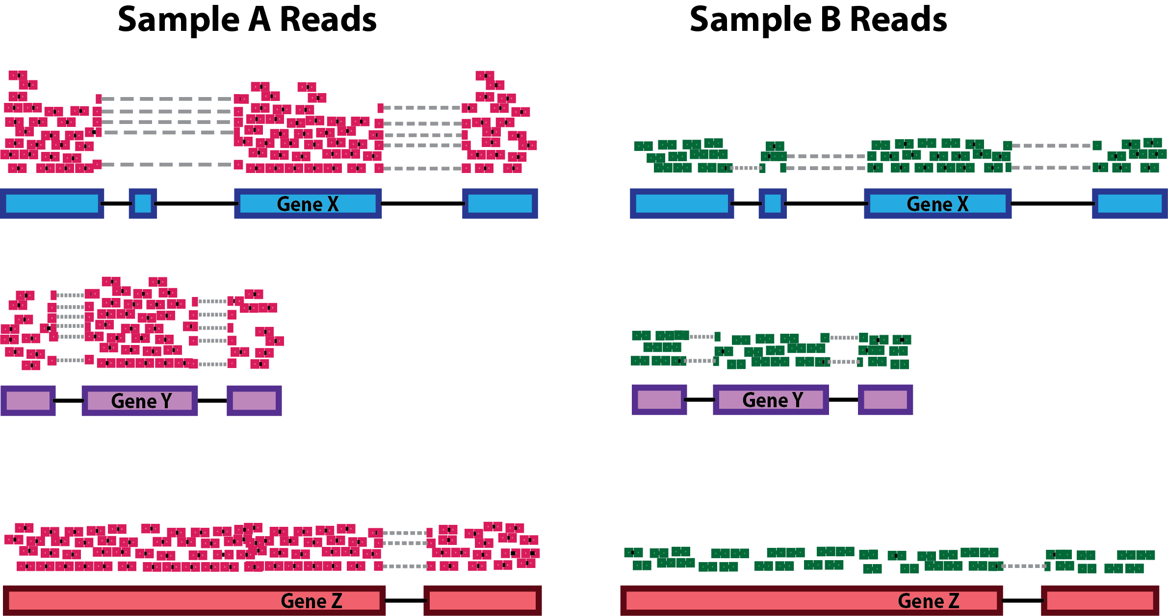
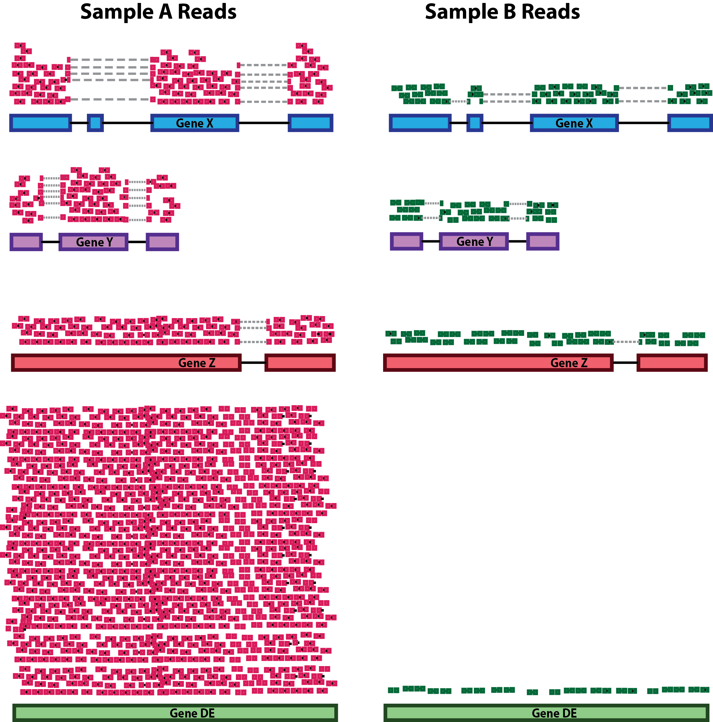
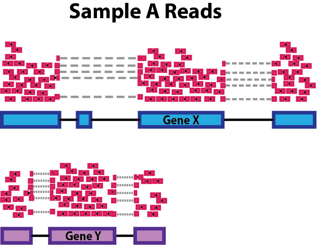
class: center, middle, inverse, title-slide # Data Preprocessing ## Workshop on RNA-Seq ### <b>Roy Francis</b> | 04-Dec-2020 ### NBIS, SciLifeLab --- exclude: true count: false <link href="https://fonts.googleapis.com/css?family=Roboto|Source+Sans+Pro:300,400,600|Ubuntu+Mono&amp;subset=latin-ext" rel="stylesheet"> <link rel="stylesheet" href="https://use.fontawesome.com/releases/v5.3.1/css/all.css" integrity="sha384-mzrmE5qonljUremFsqc01SB46JvROS7bZs3IO2EmfFsd15uHvIt+Y8vEf7N7fWAU" crossorigin="anonymous"> <!-- ------------ Only edit title, subtitle & author above this ------------ --> --- name: raw ## Raw data - Raw count table ``` ## DSSd00_1 DSSd00_2 DSSd00_3 DSSd07_1 DSSd07_2 DSSd07_3 ## ENSMUSG00000102693 0 0 0 0 0 0 ## ENSMUSG00000064842 0 0 0 0 0 0 ## ENSMUSG00000051951 0 1 2 0 3 2 ## ENSMUSG00000102851 0 0 0 0 0 0 ## ENSMUSG00000103377 0 0 0 0 0 0 ## ENSMUSG00000104017 0 0 0 0 0 0 ``` - Metadata ``` ## SampleName SampleID No Model Day Group Replicate ## DSSd00_1 DSSd00_1 KI_PC1606_01 1 DSS 0 day00 1 ## DSSd00_2 DSSd00_2 KI_PC1606_02 2 DSS 0 day00 2 ## DSSd00_3 DSSd00_3 KI_PC1606_03 3 DSS 0 day00 3 ## DSSd07_1 DSSd07_1 KI_PC1606_13 13 DSS 7 day07 1 ## DSSd07_2 DSSd07_2 KI_PC1606_14 14 DSS 7 day07 2 ## DSSd07_3 DSSd07_3 KI_PC1606_15 15 DSS 7 day07 3 ``` ??? A glimpse into the count table and metadata table. It is important to make sure before any analyses that the count column names match the metadata row names exactly. Make sure the column in both tables are of the correct data type; ie; numbers are numeric and groups are factors. --- name: pp ## Filtering - Remove genes and samples with low counts ```r cf1 <- cr[rowSums(cr>0) >= 3, ] cf2 <- cr[rowSums(cr>3) >= 3, ] cf3 <- cr[rowSums(edgeR::cpm(cr)>5) >= 3, ] ``` - Inspect distribution <img src="slide_preprocessing_files/figure-html/unnamed-chunk-6-1.svg" style="display: block; margin: auto auto auto 0;" /> - Inspect the number of rows (genes) available after filtering ``` ## Raw: 55487, Method 1: 16099, Method 2: 11783, Method 3: 12496 ``` ??? Lowly expressed genes are removed to improve the signal-to-noise ratio. Genes not expressed in any sample can be removed completely as as they negatively affect multiple testing correction. The stringency of low count filtering can be adjusted based on the researcher's preference. It is a tradeoff between data quality vs data size. In the above example, raw data has a huge number of zeros and the distribution of over higher value counts are barely visible. Three different levels of low count filtering are shown. In method 1, the detection limit is set at 1 count, ie; any value above 0 is considered as an expressed gene. And we aim to have expression in atleast 3 samples. In method 2, the detection limit is set at 3 counts, ie; any value above 3 is considered an expressed gene. A value below 3 is considered noise and is disregarded. And we aim to have 3 count expression in atleast 3 samples. Note that changing the minimum limit of detection has a dramatic effect on the count distribution. Notice how many rows (genes) are discarded. In method 3, the limit of detection is a bit less subjective. A count that is greater than 5 count per million reads is considered a positive detection. This is a stringent and fairly robust method at the expense of losing the most number of genes. --- name: norm-1 ## Normalisation .pull-left-50[ - Make counts comparable across samples - Control for sequencing depth  ``` ## A B A_tc B_tc ## x 20 6 0.33 0.38 ## y 25 6 0.42 0.38 ## z 15 4 0.25 0.25 ``` ] ??? Normalisation of raw count data is necessary to make samples comparable. The comparison may be within sample, within groups, between groups and possibly between studies. **Total count normalisation** Imagine two samples A and B with three genes x, y and z. A has higher counts than B. Are the genes highly expressed in A? Probably not. A was sequenced deeper which resulted in more reads overall. Controlling for sequencing depth is one of the the first steps with normalisation. Total count normalisation controls for sequencing depth. See columns A_tc and B_tc for the count values after total count normalisation. If the total number of starting mRNA is comparable between samples, then this value reflects absolute expression for each gene. Quantile normalisation, Upper quartile normalisation and Median normalisation all work in a similar way. Rather than the total count, a high quantile value or the median is used. -- .pull-right-50[ - Control for compositional bias  ``` ## A B A_tc B_tc ## x 0 20 0.00 0.39 ## y 25 25 0.18 0.49 ## z 15 4 0.11 0.08 ## de 100 2 0.71 0.04 ``` ] ??? **Controlling for compositional bias** In another scenario, imagine the same two samples and four genes x,y,z and de. This time, both samples are sequenced to the same depth and the gene de is highly overexpressed in A than in B. Now, look at the total count normalised value for gene y. They have different normalised values in A and B although A and B had identical expression for gene y. This effect of few highly overexpressed genes seemingly changing the relative expression of other genes is called compositional bias. --- name: norm-2 ## Normalisation - Make counts comparable across features (genes) .size-60[] ``` ## counts gene_length norm_counts ## x 50 10 5 ## y 25 5 5 ``` -- - Bring counts to a human-friendly scale ??? **Controlling for gene length** For two genes X and Y within a sample A, the longer gene will produce more reads than the shorter gene. For comparing expression of these two genes to each other, they need to be controlled for gene length. In this example, gene x has higher counts than y. But when controlled for gene length, they both have the same expression. **Counts per million reads** The last point with normalisation is to bring the numbers to a human friendly scale. This the reason for the per million part of CPM, RPKM etc. --- name: norm-3a ## Normalisation **Normalisation by library size** - Assumes total expression is the same under different experimental conditions - Methods include TC, RPKM, FPKM, TPM - RPKM, FPKM and TPM control for sequencing depth and gene length - Total number of RPKM/FPKM normalized counts for each sample will be different, therefore, you cannot compare the normalized counts for each gene equally between samples. - TPM enables better comparison between samples because total per sample sums to equal value ``` ## A B len A_rpm B_rpm A_rpkm B_rpkm A_rpk B_rpk A_tpm B_tpm ## x 20 6 20000 408163 222222 20.41 11.11 0.001000 0.00030 493827 153846 ## y 25 6 40000 510204 222222 12.76 5.56 0.000625 0.00015 308642 76923 ## z 4 15 10000 81633 555556 8.16 55.56 0.000400 0.00150 197531 769231 ## sum 49 27 70000 1000000 1000000 41.33 72.23 0.002025 0.00195 1000000 1000000 ``` ??? Normalisation strategies can be roughly grouped into four approaches: Normalisation by library size, normalisation by distribution, normalisation by testing and normalisation using controls. Normalisation by library size is the most basic. TPM is probably the only method that must be used. **RPKM** RPKM in each sample sums up to different totals which make it hard to compare a gene from one sample to another sample. ``` RPM = count / (total_counts / 10^6) RPKM = RPM / transcript_length ``` **TPM** TPM in every sample sums up to 1 million. This makes it easier to compare a gene from one sample to another. ``` RPK = count / transcript length TPM = (RPK * 10^6)/total_RPK ``` --- name: norm-3b ## Normalisation **Normalisation by distribution** - Assumes technical effects are same for DE and non-DE genes - Assumes number of over and under-expressed genes are roughly same across conditions - Corrects for compositional bias - Methods include Q, UQ, M, RLE, TMM, MRN - `edgeR::calcNormFactors()` implements TMM, TMMwzp, RLE & UQ - `DESeq2::estimateSizeFactors()` implements median ratio method (RLE) - Does not correct for gene length - **[geTMM](https://bmcbioinformatics.biomedcentral.com/articles/10.1186/s12859-018-2246-7)** is gene length corrected TMM ``` ## A B len ref A_ratio B_ratio A_mrn B_mrn ## x 20 6 20000 10.95 1.83 0.55 10.928962 10.90909 ## y 25 6 40000 12.25 2.04 0.49 13.661202 10.90909 ## z 4 15 10000 7.75 0.52 1.94 2.185792 27.27273 ``` .citation[ .cite[<i class="fas fa-link"></i> Evans, Ciaran, Johanna Hardin, and Daniel M. Stoebel. "Selecting between-sample RNA-Seq normalization methods from the perspective of their assumptions." [Briefings in bioinformatics (2017)](https://arxiv.org/abs/1609.00959)] ] ??? **MRN** MRN method assumes most samples are not differentially expressed - Find a reference sample for each gene. - Divide each count by the reference sample to create a ratio - Compute median of this ratio for each sample - Divide counts by this median ratio Normalisation by distribution controls for composition bias. Most software use a mix of different approaches. --- name: norm-3c ## Normalisation **Normalisation by testing** - A more robust version of normalisation by distribution. - A set of non-DE genes are detected through hypothesis testing - Tolerates a larger difference in number of over and under expressed genes between conditions - Methods include PoissonSeq, DEGES -- **Normalisation using Controls** - Assumes controls are not affected by experimental condition and technical effects are similar to all other genes - Useful in conditions with global shift in expression - Controls could be house-keeping genes or spike-ins - Methods include RUV, CLS -- **Stabilizing variance** - Variance is stabilised across the range of mean values - Methods include VST, RLOG, VOOM - For use in exploratory analyses. Not for DE. - `vst()` and `rlog()` functions from *DESeq2* - `voom()` function from *Limma* converts data to normal distribution --- name: norm-4 exclude: true ## Normalisation | Method | Description | Accounted factors | Recommendation | | ---- | ---- | ---- | ---- | | CPM | counts scaled by total number of reads | sequencing depth | compare counts between replicates of the same group; NOT for within sample comparisons or DE analysis | | TPM| counts per length of transcript (kb) per million reads mapped | sequencing depth and gene length | gene count comparisons within a sample or between samples of the same sample group; NOT for DE analysis | | RPKM/FPKM | similar to TPM | sequencing depth and gene length | compare counts between genes within a sample; NOT for between sample comparisons or DE analysis | | DESeq2 MRN | counts divided by sample-specific size factors determined by median ratio of gene counts relative to geometric mean per gene | sequencing depth and RNA composition | compare counts between samples and for DE analysis; NOT for within sample comparisons | | EdgeR TMM | uses a weighted trimmed mean of the log expression ratios between samples | sequencing depth, RNA composition, and gene length | compare counts between and within samples and for DE analysis | --- name: norm-5 ## Normalisation **Recommendations** - Most tools use a mix of many different normalisations - For DGE using DGE R packages (DESeq2, edgeR, Limma etc), use raw counts - For visualisation (PCA, clustering, heatmaps etc), use VST or RLOG - For own analysis with gene length correction, use TPM (maybe geTMM?) - Custom solutions: spike-ins/house-keeping genes -- .citation[ .cite[<i class="fas fa-link"></i> Dillies, Marie-Agnes, *et al*. "A comprehensive evaluation of normalization methods for Illumina high-throughput RNA sequencing data analysis." [Briefings in bioinformatics 14.6 (2013): 671-683](https://www.ncbi.nlm.nih.gov/pubmed/22988256)] ] --- # Acknowledgements - [Normalising RNA-seq data](https://www.ebi.ac.uk/sites/ebi.ac.uk/files/content.ebi.ac.uk/materials/2012/121029_HTS/ernest_turro_normalising_rna-seq_data.pdf) by Ernest Turro - RNA-seq analysis [Bioconductor vignette](http://master.bioconductor.org/packages/release/workflows/vignettes/rnaseqGene/inst/doc/rnaseqGene.html) --- name: end_slide class: end-slide, middle count: false # Thank you. Questions? .end-text[ <p>R version 4.0.3 (2020-10-10)<br><p>Platform: x86_64-pc-linux-gnu (64-bit)</p><p>OS: Ubuntu 18.04.5 LTS</p><br> <hr> <span class="small">Built on : <i class='fa fa-calendar' aria-hidden='true'></i> 04-Dec-2020 at <i class='fa fa-clock-o' aria-hidden='true'></i> 00:13:10</span> <b>2020</b> • [SciLifeLab](https://www.scilifelab.se/) • [NBIS](https://nbis.se/) ]