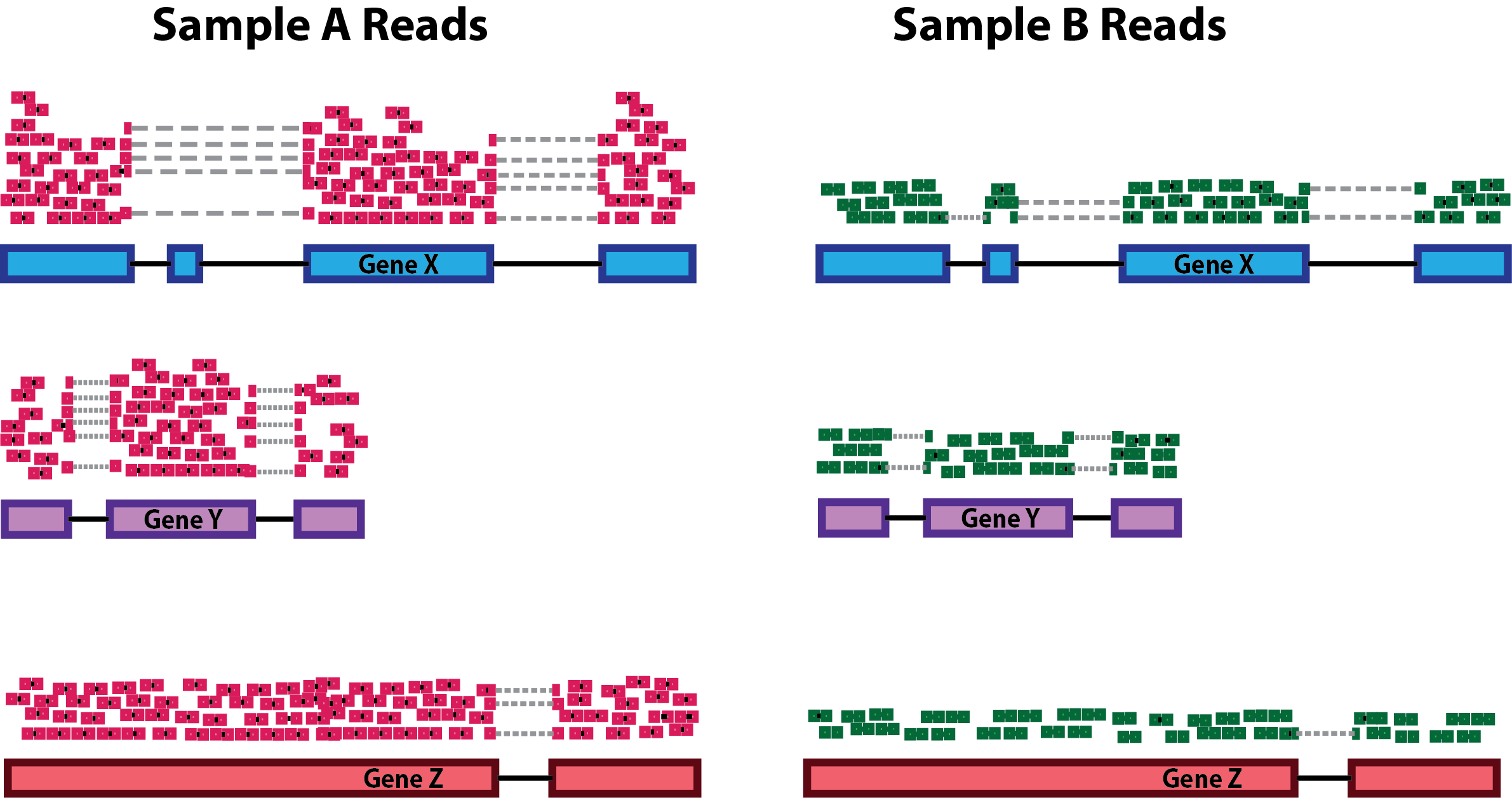
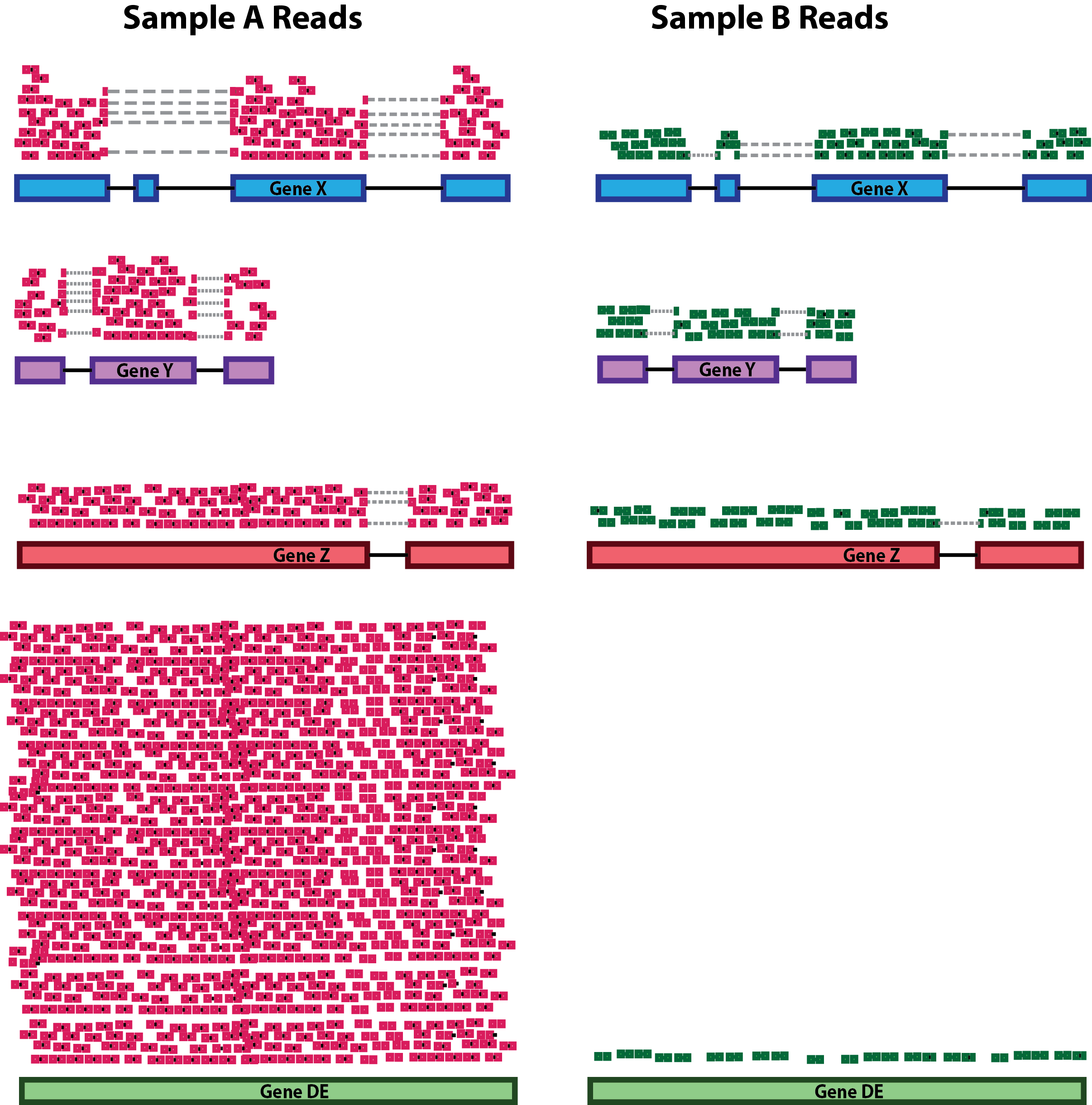
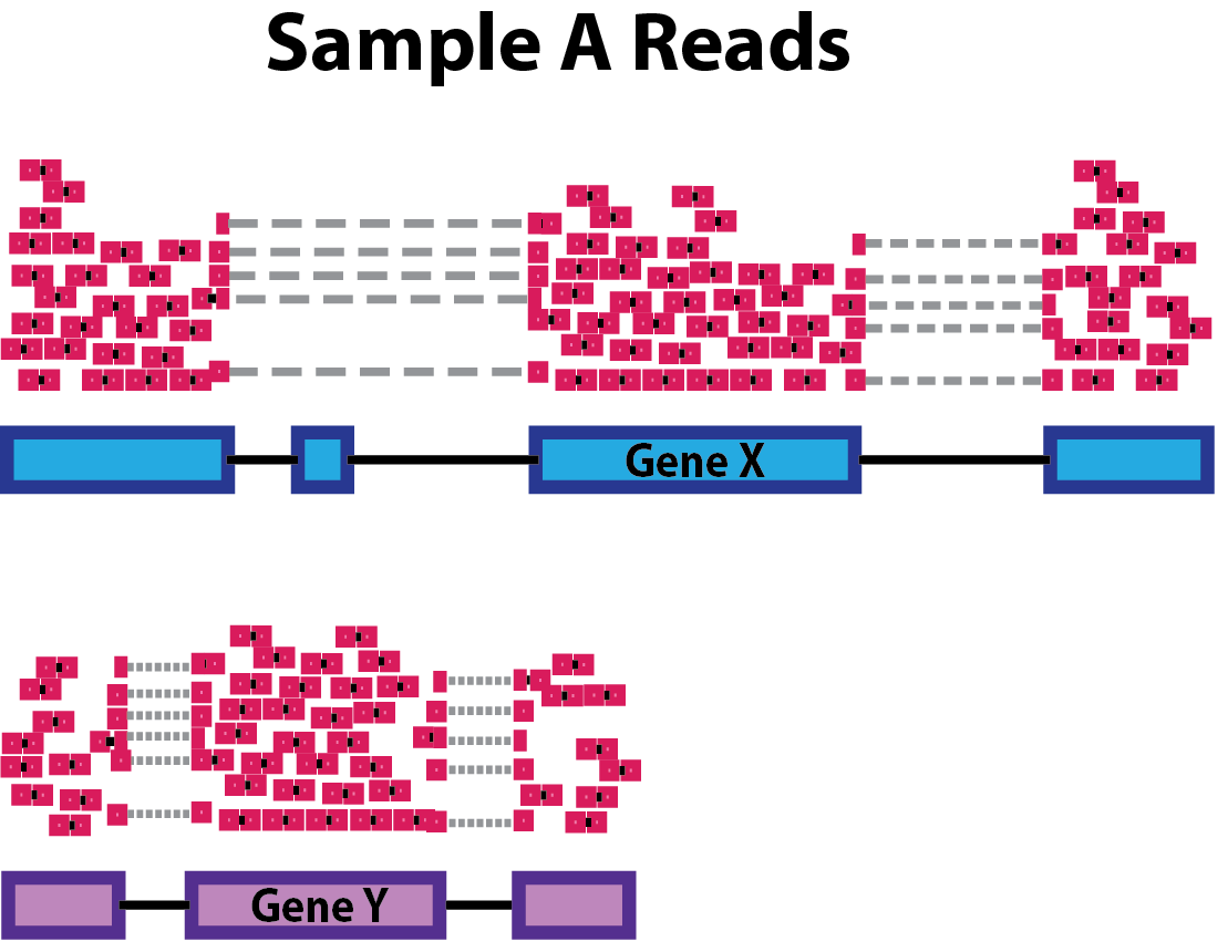
Differential Gene Expression Workflow

class: center, middle, inverse, title-slide

# Differential Gene Expression Workflow
## Workshop on RNA-Seq
### Roy Francis | 03-Jun-2019

---

exclude: true
count: false

---
name: content
class: spaced

## Contents

* [Preprocessing](#pp)
* [Normalisation](#norm-1)
* [Exploratory](#eda-cor)
* [DGE](#dge)

---
name: raw

## Raw data

- Raw count table

```
##                 Sample_1 Sample_2 Sample_3 Sample_4 Sample_5 Sample_6
## ENSG00000000003      321      303      204      492      455      359
## ENSG00000000005        0        0        0        0        0        0
## ENSG00000000419      696      660      472      951      963      689
## ENSG00000000457       59       54       44      109       73       66
## ENSG00000000460      399      405      236      445      454      374
## ENSG00000000938        0        0        0        0        0        1
```

- Metadata

```
##          Sample_ID Sample_Name Time Replicate Cell
## Sample_1  Sample_1        t0_A   t0         A A431
## Sample_2  Sample_2        t0_B   t0         B A431
## Sample_3  Sample_3        t0_C   t0         C A431
## Sample_4  Sample_4        t2_A   t2         A A431
## Sample_5  Sample_5        t2_B   t2         B A431
## Sample_6  Sample_6        t2_C   t2         C A431
```

---
name: pp

## Preprocessing

- Remove genes and samples with low counts

```r
cf1 <- cr[rowSums(cr>0) >= 2, ]
cf2 <- cr[rowSums(cr>5) >= 2, ]
cf3 <- cr[rowSums(edgeR::cpm(cr)>1) >= 2, ]
```

- Inspect distribution

- Inspect the number of rows

```
## Raw: 59573, Method 1: 24194, Method 2: 16519, Method 3: 14578
```

---
name: norm-1

## Normalisation

.pull-left-50[
- Make counts comparable across samples
- Control for sequencing depth

![](images/normalization_methods_depth.png)

```
##   s1 s2 s1_tc s2_tc
## x 20  6  0.33  0.38
## y 25  6  0.42  0.38
## z 15  4  0.25  0.25
```
]

.pull-right-50[
- Control for compositional bias
![](images/normalization_methods_composition.png)

```
##     s1 s2 s1_tc s2_tc
## x   20 20  0.12  0.39
## y   25 25  0.16  0.49
## z   15  4  0.09  0.08
## de 100  2  0.62  0.04
```
]

---
name: norm-2

## Normalisation

- Make counts comparable across features (genes)
.size-60[![](images/normalization_methods_length.png)]

```
##   counts gene_length norm_counts
## 1     50          10           5
## 2     25           5           5
```

- Bring counts to a human-friendly scale

---
name: norm-3

## Normalisation

- CPM, RPKM, FPKM, TPM, RLE, MRN, Q, UQ, TMM, VST, RLOG, VOOM ... Too many...

- **CPM**: Controls for sequencing depth when dividing by total count. Not for within-sample comparison or DE.

- **RPKM/FPKM**: Controls for sequencing depth and gene length. Good for technical replicates, not good for sample-sample due to compositional bias. Assumes total RNA output is same in all samples. Not for DE.

- **TPM**: Similar to RPKM/FPKM. Corrects for sequencing depth and gene length. Also comparable between samples but no correction for compositional bias.

- **TMM/RLE/MRN**: Improved assumption: The output between samples for a core set only of genes is similar. Corrects for compositional bias. Used for DE. RLE and MRN are very similar and correlates well with sequencing depth. `edgeR::calcNormFactors()` implements TMM, TMMwzp, RLE & UQ. `DESeq2::estimateSizeFactors` implements median ratio method (RLE). Does not correct for gene length.

- **VST/RLOG/VOOM**: Variance is stabilised across the range of mean values. For use in exploratory analyses. Not for DE. `vst()` and `rlog()` functions from *DESeq2*. `voom()` function from *Limma* converts data to normal distribution.

- **[geTMM](https://bmcbioinformatics.biomedcentral.com/articles/10.1186/s12859-018-2246-7)**: Gene length corrected TMM.

.citation[
.cite[ Dillies, Marie-Agnes, *et al*. "A comprehensive evaluation of normalization methods for Illumina high-throughput RNA sequencing data analysis." [Briefings in bioinformatics 14.6 (2013): 671-683](https://www.ncbi.nlm.nih.gov/pubmed/22988256)] 
.cite[ Evans, Ciaran, Johanna Hardin, and Daniel M. Stoebel. "Selecting between-sample RNA-Seq normalization methods from the perspective of their assumptions." [Briefings in bioinformatics (2017)](https://arxiv.org/abs/1609.00959)] 
]

---
name: norm-4

## Normalisation

**Recommendations**

- For DGE using DGE R packages (DESeq2, edgeR, Limma etc), use raw counts
- For visualisation (PCA, clustering, heatmaps etc), use VST or RLOG
- For own analysis with gene length correction, use TPM (maybe geTMM?)
- Other solutions: spike-ins/house-keeping genes

---
name: eda-cor

## Exploratory | Correlation

* Correlation between samples

```r
dmat <- as.matrix(cor(cv,method="spearman"))
pheatmap::pheatmap(dmat,border_color=NA,annotation_col=mr[,"Time",drop=F],
 annotation_row=mr[,"Time",drop=F],annotation_legend=T)
```

---
name: eda-dist

## Exploratory | Distance

* Similarity between samples

```r
dmat <- as.matrix(dist(t(cv)))
pheatmap(dmat,border_color=NA,annotation_col=mr[,"Time",drop=F],
 annotation_row=mr[,"Time",drop=F],annotation_legend=T)
```

---
name: eda-pca

## Exploratory | PCA

* Relationship between samples

.pull-left-40[
<img src="presentation_dge_files/figure-html/unnamed-chunk-17-1.svg" style="display: block; margin: auto auto auto 0;" />
]

.pull-right-60[
<img src="presentation_dge_files/figure-html/unnamed-chunk-18-1.svg" style="display: block; margin: auto auto auto 0;" />

]

---
name: dge

## DGE

* Create the DESeq2 object

```r
library(DESeq2)
mr$Time <- factor(mr$Time)
d <- DESeqDataSetFromMatrix(countData=cf,colData=mr,design=~Time)
d
```

```
## class: DESeqDataSet 
## dim: 14578 12 
## metadata(1): version
## assays(1): counts
## rownames(14578): ENSG00000000003 ENSG00000000419 ...
##   ENSG00000266865 ENSG00000266876
## rowData names(0):
## colnames(12): Sample_1 Sample_2 ... Sample_11 Sample_12
## colData names(5): Sample_ID Sample_Name Time Replicate Cell
```

* Model must be factors

- `~var`
- `~covar+var`

---
name: dge-sf

## DGE | Size factors

* Normalisation factors are computed

```r
d <- DESeq2::estimateSizeFactors(d,type="ratio")
sizeFactors(d)
```

```
##  Sample_1  Sample_2  Sample_3  Sample_4  Sample_5  Sample_6  Sample_7 
## 0.9003753 0.8437393 0.5106445 1.1276451 1.0941383 0.8133849 0.7553903 
##  Sample_8  Sample_9 Sample_10 Sample_11 Sample_12 
## 1.1744008 1.0189325 1.3642797 1.2325485 1.8555904
```

---
name: dge-dispersion

## DGE | Dispersion

* We need a measure variability of gene counts

```r
dm <- apply(cd,1,mean)
dv <- apply(cd,1,var)
cva <- function(x) sd(x)/mean(x)
dc <- apply(cd,1,cva)
```

* Dispersion is a measure of variability in gene expression for a given mean

---
name: dge-dispersion-2

## DGE | Dispersion

* D is unreliable for low mean counts
* Genes with similar mean values must have similar dispersion
* Estimate likely (ML) dispersion for each gene based on counts
* Fit a curve through the gene-wise estimates
* Shrink dispersion towards the curve

```r
d <- DESeq2::estimateDispersions(d)
{par(mar=c(4,4,1,1))
plotDispEsts(d)}
```

---
name: dge-test

## DGE | Test

* Log2 fold changes changes are computed after GLM fitting

```r
dg <- nbinomWaldTest(d)
resultsNames(dg)
```

```
## [1] "Intercept"      "Time_t2_vs_t0"  "Time_t24_vs_t0" "Time_t6_vs_t0"
```

* Use `results()` to customise/return results
  * Set coefficients using `contrast` or `name`
  * Filtering by fold change using `lfcThreshold`
  * `cooksCutoff` removes outliers
  * `independentFiltering`
  * `pAdjustMethod`
  * `alpha`

---
name: dge-test-2

## DGE | Test

```r
res1 <- results(dg,name="Time_t2_vs_t0",alpha=0.05)
summary(res1)
```

```
## 
## out of 14578 with nonzero total read count
## adjusted p-value < 0.05
## LFC > 0 (up) : 413, 2.8%
## LFC < 0 (down) : 696, 4.8%
## outliers [1] : 0, 0%
## low counts [2] : 2261, 16%
## (mean count < 26)
## [1] see 'cooksCutoff' argument of ?results
## [2] see 'independentFiltering' argument of ?results
```

---
name: dge-test-3

## DGE | Test

```r
head(res1)
```

```
## log2 fold change (MLE): Time t2 vs t0 
## Wald test p-value: Time t2 vs t0 
## DataFrame with 6 rows and 6 columns
## baseMean log2FoldChange lfcSE
## <numeric> <numeric> <numeric>
## ENSG00000000003 490.017213130775 0.220619809383656 0.112761083788383
## ENSG00000000419 817.780657499214 0.0592719659601406 0.101481284662652
## ENSG00000000457 82.078767893562 0.207748623172909 0.220404896514001
## ENSG00000000460 356.07160020304 -0.129186381676072 0.115139182335103
## ENSG00000001036 919.606750211436 0.0288826917736355 0.0851500691928604
## ENSG00000001084 529.593965301543 0.211964772147193 0.0929810563117334
## stat pvalue padj
## <numeric> <numeric> <numeric>
## ENSG00000000003 1.95652437854969 0.0504034135093116 0.263505451695327
## ENSG00000000419 0.584067950629267 0.559174596319379 0.830262316260423
## ENSG00000000457 0.942577168015466 0.34589722283592 0.689945926100409
## ENSG00000000460 -1.12200190288033 0.2618616308297 0.612624613846088
## ENSG00000001036 0.33919751384133 0.734460942036292 0.909638554355053
## ENSG00000001084 2.27965545408033 0.0226281312376226 0.159263252830742
```

* Use `lfcShrink()` to correct fold changes for high dispersion genes

---

# Acknowledgements

* [Normalising RNA-seq data](https://www.ebi.ac.uk/sites/ebi.ac.uk/files/content.ebi.ac.uk/materials/2012/121029_HTS/ernest_turro_normalising_rna-seq_data.pdf) by Ernest Turro  
* RNA-seq analysis [Bioconductor vignette](http://master.bioconductor.org/packages/release/workflows/vignettes/rnaseqGene/inst/doc/rnaseqGene.html)
* [DGE Workshop](https://github.com/hbctraining/DGE_workshop/tree/master/lessons) by HBC training

---
name: end_slide
class: end-slide, middle
count: false

# Thank you. Questions?

.end-text[
R version 3.5.2 (2018-12-20) Platform: x86_64-pc-linux-gnu (64-bit)OS: Ubuntu 18.04.2 LTS

<hr>

Built on : 03-Jun-2019 at 22:54:57

2019 • [SciLifeLab](https://www.scilifelab.se/) • [NBIS](https://nbis.se/)
]