Tidy work in Tidyverse

RaukR 2026 • Data Science With R

Marcin Kierczak

18-Aug-2026

Learning Outcomes

When this module is complete, you will:

know what tidyverse is and a bit about its history
be able to use different pipes, including advanced ones and placeholders
know whether the data you work with are tidy
will be able to load, debug and tidy your data
understand how to combine data sets using join_*
be aware of useful packages within tidyverse

Tidyverse — what is it all about?

tidyverse is a collection of packages 📦,
created by Hadley Wickham,
has became a de facto standard in data analyses,
a philosophy of programming or a programming paradigm: everything is about the 🌊 flow of 🧹 tidy data.

`?(Tidyverse OR !Tidyverse)`

Warning

☠️ There are still some people out there talking about the tidyverse curse though… ☠️

Navigating the balance between base R and the tidyverse is a challenge to learn.
- Robert A. Muenchen

Typical Tidyverse Workflow

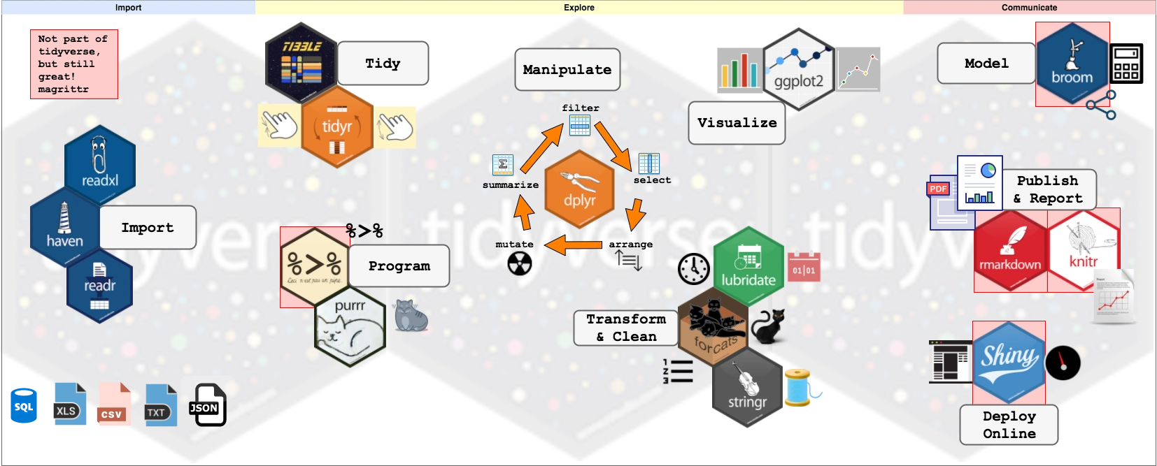
Source: http://www.storybench.org/getting-started-with-tidyverse-in-r/

Introduction to Pipes or Let My Data Flow 🌊

Rene Magritt, La trahison des images, Wikimedia Commons

magrittr package — tidyverse and beyond
the %>% pipe
- x %>% f $\equiv$ f(x)
- x %>% f(y) $\equiv$ f(x, y)
- x %>% f %>% g %>% h $\equiv$ h(g(f(x)))

Introduction to Pipes

Instead of writing this:

result <- head(iris, n=3)

write this:

iris %>% head(n=3)

  Sepal.Length Sepal.Width Petal.Length Petal.Width Species
1          5.1         3.5          1.4         0.2  setosa
2          4.9         3.0          1.4         0.2  setosa
3          4.7         3.2          1.3         0.2  setosa

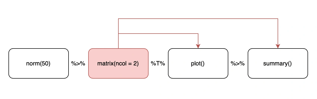
Other Types of Pipes — `%T>%`

Provided by magritter, not in tidyverse
When you call a function for its side effects

rnorm(50) %>% 
  matrix(ncol = 2) %>% 
  plot() %>% 
  summary()

Length  Class   Mode 
     0   NULL   NULL

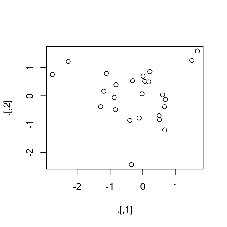
Other Types of Pipes — `%T>%`

rnorm(50) %>% 
  matrix(ncol = 2) %T>% 
  plot() %>% 
  summary()

       V1                V2          
 Min.   :-2.0793   Min.   :-1.78298  
 1st Qu.:-0.6641   1st Qu.:-0.57008  
 Median :-0.1182   Median :-0.05799  
 Mean   :-0.1180   Mean   :-0.09141  
 3rd Qu.: 0.3785   3rd Qu.: 0.33888  
 Max.   : 1.3904   Max.   : 1.96132

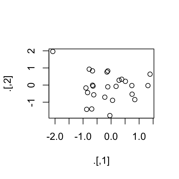
Other Types of `magrittr` Pipes — `%$%`

iris %>% cor(Sepal.Length, Sepal.Width)

Error:
! object 'Sepal.Width' not found

We need the %$% pipe with exposition of variables:

iris %$% cor(Sepal.Length, Sepal.Width)

[1] -0.1175698

This is because cor function does not have the x (data) argument – the very first argument of a pipe-friendly function.

Other Types of `magrittr` Pipes — %<>%

It exists but can lead to somewhat confusing code! ☠️

x %<>% f $\equiv$ x <- f(x)

M <- matrix(rnorm(16), nrow=4); M %<>% colSums(); M

[1] -2.9134619 -0.7215132  1.2680168 -3.9148186

Native R pipe

From R >= 4.1.0 we have a native |> pipe that is fasterm than %>%, dependency-free and native but has less rich placeholders mechanism.

c(1,2,3,4,5) |> mean()

[1] 3

a placeholder _ is available but ☠️ only for named arguments.

mtcars |> lm(mpg ~ disp, data = _)


Call:
lm(formula = mpg ~ disp, data = mtcars)

Coefficients:
(Intercept)         disp  
   29.59985     -0.04122

Placeholders in `magrittr` Pipes

Sometimes we want to pass the resulting data to other than the first argument of the next function in chain. magritter provides placeholder mechanism for this:

x %>% f(y, .) $\equiv$ f(y, x),
x %>% f(y, z = .) $\equiv$ f(y, z = x)

M <- rnorm(4) %>% matrix(nrow = 2)
M %>% `%*%`(., .)

           [,1]       [,2]
[1,]  0.9802302 -0.1619007
[2,] -0.3268864  0.7086858

Placeholders for nested expressions

But for nested expressions:

x %>% f(a = p(.), b = q(.)) $\equiv$ f(x, a = p(x), b = q(x))

x %>% {f(a = p(.), b = q(.))} $\equiv$ f(a = p(x), b = q(x))

print_M_summ <- function(nrow, ncol) paste0('Matrix M has: ', nrow, ' rows and ', ncol, ' cols.')
M %>% {print_M_summ(nrow(.), ncol(.))}

[1] "Matrix M has: 2 rows and 2 cols."

Placeholders – unary functions

We can even use placeholders as the first element of a pipe:

f <- . %>% sin %>% cos
f

Functional sequence with the following components:

 1. sin(.)
 2. cos(.)

Use 'functions' to extract the individual functions.

and, indeed the f function works:

7 %>% f

[1] 0.7918362

Time to do Lab 1.1

Tibbles

tibble is one of the unifying features of tidyverse,
it is a better data.frame realization,
objects data.frame can be coerced to tibble using as_tibble()

Convert `data.frame` to `tibble`

as_tibble(iris)

# A tibble: 150 × 5
   Sepal.Length Sepal.Width Petal.Length Petal.Width Species
          <dbl>       <dbl>        <dbl>       <dbl> <fct>  
 1          5.1         3.5          1.4         0.2 setosa 
 2          4.9         3            1.4         0.2 setosa 
 3          4.7         3.2          1.3         0.2 setosa 
 4          4.6         3.1          1.5         0.2 setosa 
 5          5           3.6          1.4         0.2 setosa 
 6          5.4         3.9          1.7         0.4 setosa 
 7          4.6         3.4          1.4         0.3 setosa 
 8          5           3.4          1.5         0.2 setosa 
 9          4.4         2.9          1.4         0.2 setosa 
10          4.9         3.1          1.5         0.1 setosa 
# ℹ 140 more rows

Tibbles from scratch with `tibble`

  tibble(
    x = 1,          # recycling
    y = runif(50), 
    z = x + y^2,
    outcome = rnorm(50)
  )

# A tibble: 50 × 4
       x       y     z outcome
   <dbl>   <dbl> <dbl>   <dbl>
 1     1 0.280    1.08   0.145
 2     1 0.391    1.15  -0.215
 3     1 0.465    1.22  -0.529
 4     1 0.546    1.30  -2.63 
 5     1 0.273    1.07  -0.551
 6     1 0.957    1.92   1.19 
 7     1 0.181    1.03  -1.03 
 8     1 0.847    1.72   0.624
 9     1 0.370    1.14  -1.41 
10     1 0.00178  1.00  -0.118
# ℹ 40 more rows

More on Tibbles

When you print a tibble:
- all columns that fit the screen are shown,
- only the first 10 rows are shown,
- data type for each column is shown.

as_tibble(cars)

# A tibble: 50 × 2
   speed  dist
   <dbl> <dbl>
 1     4     2
 2     4    10
 3     7     4
 4     7    22
 5     8    16
 6     9    10
 7    10    18
 8    10    26
 9    10    34
10    11    17
# ℹ 40 more rows

Tibble printing options

my_tibble %>% print(n = 50, width = Inf),
options(tibble.print_min = 15, tibble.print_max = 25),
options(dplyr.print_min = Inf),
options(tibble.width = Inf)

Subsetting Tibbles

vehicles will be our tibble version of cars

vehicles <- as_tibble(cars[1:5,])

We can access data like this:

vehicles[['speed']]
vehicles[[1]]
vehicles$speed

[1] 4 4 7 7 8
[1] 4 4 7 7 8
[1] 4 4 7 7 8

Or, alternatively, using placeholders:

vehicles %>% .$speed
vehicles %>% .[['speed']]
vehicles %>% .[[1]]

Note! Not all old R functions work with tibbles, than you have to use as.data.frame(my_tibble).

Partial Matching

cars <- cars[1:5,]; colnames(vehicles)

[1] "speed" "dist"

cars$spe      # partial matching

[1] 4 4 7 7 8

vehicles$spe  # no partial matching

Warning: Unknown or uninitialised column: `spe`.

NULL

Non-existing Columns

cars$gear

NULL

vehicles$gear

Warning: Unknown or uninitialised column: `gear`.

NULL

Time to do Lab 1.2

Loading Data

In tidyverse you import data using readr package (relying on fast vroom engine) that provides a number of useful data import functions:

read_delim() a generic function for reading x-delimited files. There are a number of convenience wrappers:
- read_csv() used to read comma-delimited files,
- read_csv2() reads semicolon-delimited files, read_tsv() that reads tab-delimited files.
read_fwf for reading fixed-width files with its wrappers:
- fwf_widths() for width-based reading,
- fwf_positions() for positions-based reading and
- read_table() for reading white space-delimited fixed-width files.
read_log() for reading Apache-style logs.

Loading Data

The most commonly used read_csv() has some familiar arguments like:

skip – to specify the number of rows to skip (headers),
col_names – to supply a vector of column names,
comment – to specify what character designates a comment,
na – to specify how missing values are represented.

Under the Hood – `parse_*` Functions

Under the hood, data-reading functions use parse_* functions:

parse_double("42.24")

[1] 42.24

parse_number("272'555'849,55", 
             locale = locale(decimal_mark = ",", 
                             grouping_mark = "'"
                            )
             )

[1] 272555850

parse_number(c('100%', 'price: 500$', '21sek', '42F'))

[1] 100 500  21  42

Parsing Strings

Strings can be represented in different encodings:

text1 <- 'På en ö är en å'
text2 <- 'Zażółć gęślą jaźń'

charToRaw(text2)
parse_character(text1, locale = locale(encoding = 'UTF-8'))
guess_encoding(charToRaw(text2))

 [1] 5a 61 c5 bc c3 b3 c5 82 c4 87 20 67 c4 99 c5 9b 6c c4 85 20 6a 61 c5 ba c5
[26] 84
[1] "På en ö är en å"
# A tibble: 2 × 2
  encoding     confidence
  <chr>             <dbl>
1 UTF-8              1   
2 windows-1252       0.24

Parsing Factors

R is using factors to represent categorical variables.
Supply known levels to parse_factor so that it warns you when an unknown level is present in the data:

landscapes <- c('mountains', 'swamps', 'shore')
parse_factor(c('mountains', 'plains', 'shore', 'swamps'), 
             levels = landscapes)

[1] mountains <NA>      shore     swamps   
attr(,"problems")
# A tibble: 1 × 4
    row   col expected           actual
  <int> <int> <chr>              <chr> 
1     2    NA value in level set plains
Levels: mountains swamps shore

Other Parsing Functions

parse_

vector, time, number, logical, integer, double, character, date, datetime,
guess

guess_parser("2018-06-11 09:00:00")
parse_guess("2018-06-11 09:00:00")

guess_parser(c(1, 2.3, "23$", "54%"))
parse_guess(c(1, 2.3, "23$", "54%"))

[1] "datetime"
[1] "2018-06-11 09:00:00 UTC"
[1] "character"
[1] "1"   "2.3" "23$" "54%"

Writing to a File

The readr package also provides functions useful for writing tibbled data into a file:

write_csv()
write_tsv()
write_excel_csv()

They always save:

Text in UTF-8,
Dates in ISO8601

But saving in csv (or tsv) does mean you loose information about the type of data in particular columns. You can avoid this by using:

write_rds() and read_rds() to read/write objects in R binary rds format,
Tse write_feather() and read_feather() from package feather to read/write objects in a fast binary format that other programming languages can access.

Time to do Lab 1.3

Basic Data Transformations with `dplyr`

Let us create a tibble:

jewels <- as_tibble(diamonds) |> head()
jewels[1:5,]

# A tibble: 5 × 10
  carat cut     color clarity depth table price     x     y     z
  <dbl> <ord>   <ord> <ord>   <dbl> <dbl> <int> <dbl> <dbl> <dbl>
1  0.23 Ideal   E     SI2      61.5    55   326  3.95  3.98  2.43
2  0.21 Premium E     SI1      59.8    61   326  3.89  3.84  2.31
3  0.23 Good    E     VS1      56.9    65   327  4.05  4.07  2.31
4  0.29 Premium I     VS2      62.4    58   334  4.2   4.23  2.63
5  0.31 Good    J     SI2      63.3    58   335  4.34  4.35  2.75

Picking Observations using `filter()`

jewels |> filter(cut == 'Ideal' | cut == 'Premium', carat >= 0.23) |> head()

# A tibble: 2 × 10
  carat cut     color clarity depth table price     x     y     z
  <dbl> <ord>   <ord> <ord>   <dbl> <dbl> <int> <dbl> <dbl> <dbl>
1  0.23 Ideal   E     SI2      61.5    55   326  3.95  3.98  2.43
2  0.29 Premium I     VS2      62.4    58   334  4.2   4.23  2.63

Floating point and `tidyverse`

Caution

🚤 Be careful with floating point comparisons!
🦜 Also, rows with comparison resulting in NA are skipped by default!

jewels |> filter(near(0.23, carat) | is.na(carat)) |> head(n = 4)

# A tibble: 2 × 10
  carat cut   color clarity depth table price     x     y     z
  <dbl> <ord> <ord> <ord>   <dbl> <dbl> <int> <dbl> <dbl> <dbl>
1  0.23 Ideal E     SI2      61.5    55   326  3.95  3.98  2.43
2  0.23 Good  E     VS1      56.9    65   327  4.05  4.07  2.31

Rearranging Observations using `arrange()`

jewels |> arrange(cut, carat, desc(price))

# A tibble: 6 × 10
  carat cut       color clarity depth table price     x     y     z
  <dbl> <ord>     <ord> <ord>   <dbl> <dbl> <int> <dbl> <dbl> <dbl>
1  0.23 Good      E     VS1      56.9    65   327  4.05  4.07  2.31
2  0.31 Good      J     SI2      63.3    58   335  4.34  4.35  2.75
3  0.24 Very Good J     VVS2     62.8    57   336  3.94  3.96  2.48
4  0.21 Premium   E     SI1      59.8    61   326  3.89  3.84  2.31
5  0.29 Premium   I     VS2      62.4    58   334  4.2   4.23  2.63
6  0.23 Ideal     E     SI2      61.5    55   326  3.95  3.98  2.43

Caution

The NAs always end up at the end of the rearranged tibble.

jewels |> select(color, clarity, x:z) |> head(n = 4)

# A tibble: 4 × 5
  color clarity     x     y     z
  <ord> <ord>   <dbl> <dbl> <dbl>
1 E     SI2      3.95  3.98  2.43
2 E     SI1      3.89  3.84  2.31
3 E     VS1      4.05  4.07  2.31
4 I     VS2      4.2   4.23  2.63

jewels |> select(-(x:z)) |> head(n = 5)

# A tibble: 5 × 7
  carat cut     color clarity depth table price
  <dbl> <ord>   <ord> <ord>   <dbl> <dbl> <int>
1  0.23 Ideal   E     SI2      61.5    55   326
2  0.21 Premium E     SI1      59.8    61   326
3  0.23 Good    E     VS1      56.9    65   327
4  0.29 Premium I     VS2      62.4    58   334
5  0.31 Good    J     SI2      63.3    58   335

Renaming variables

Note

rename is a variant of select, here used to rename x to var_x

jewels |> rename(var_x = x) |> head(n = 2)

# A tibble: 2 × 10
  carat cut     color clarity depth table price var_x     y     z
  <dbl> <ord>   <ord> <ord>   <dbl> <dbl> <int> <dbl> <dbl> <dbl>
1  0.23 Ideal   E     SI2      61.5    55   326  3.95  3.98  2.43
2  0.21 Premium E     SI1      59.8    61   326  3.89  3.84  2.31

Bring columns to front

Tip

use relocate() (instead of legacy everything()) to bring some columns to the front

jewels |> relocate(x:z) |> head(n = 2)
jewels |> select(x:z, everything()) |> head(n = 2) # legacy

# A tibble: 2 × 10
      x     y     z carat cut     color clarity depth table price
  <dbl> <dbl> <dbl> <dbl> <ord>   <ord> <ord>   <dbl> <dbl> <int>
1  3.95  3.98  2.43  0.23 Ideal   E     SI2      61.5    55   326
2  3.89  3.84  2.31  0.21 Premium E     SI1      59.8    61   326

And relocate is very flexible:

jewels %>%
  relocate(x:z, .after = cut)

jewels %>%
  relocate(x:z, .before = price)

Create/alter new Variables with `mutate`

jewels |> 
  mutate(p = x + z, q = p + y) |> 
  select(-(depth:price)) |> 
  head(n = 5)

# A tibble: 5 × 9
  carat cut     color clarity     x     y     z     p     q
  <dbl> <ord>   <ord> <ord>   <dbl> <dbl> <dbl> <dbl> <dbl>
1  0.23 Ideal   E     SI2      3.95  3.98  2.43  6.38  10.4
2  0.21 Premium E     SI1      3.89  3.84  2.31  6.2   10.0
3  0.23 Good    E     VS1      4.05  4.07  2.31  6.36  10.4
4  0.29 Premium I     VS2      4.2   4.23  2.63  6.83  11.1
5  0.31 Good    J     SI2      4.34  4.35  2.75  7.09  11.4

Conditional mutate

The legacy way:

iris |>
  as_tibble() |>
  mutate_if(is.numeric, scale)

should be replaced with modern across() approach:

ris |>
  as_tibble() |>
  mutate(across(where(is.numeric), scale))

Create/alter new Variables with `transmute` 🧙‍♂️

Caution

Only the transformed variables will be retained.

jewels |> transmute(carat, cut, sum = x + y + z) |>  head(n = 5)

# A tibble: 5 × 3
  carat cut       sum
  <dbl> <ord>   <dbl>
1  0.23 Ideal    10.4
2  0.21 Premium  10.0
3  0.23 Good     10.4
4  0.29 Premium  11.1
5  0.31 Good     11.4

Group and Summarize

Simple
More complex

jewels |> group_by(cut) |>  summarize(max_price = max(price),
                                      mean_price = mean(price),
                                      min_price = min(price))

# A tibble: 4 × 4
  cut       max_price mean_price min_price
  <ord>         <int>      <dbl>     <int>
1 Good            335        331       327
2 Very Good       336        336       336
3 Premium         334        330       326
4 Ideal           326        326       326

jewels |> group_by(cut, color) |>  summarize(max_price = max(price), 
                                              mean_price = mean(price), 
                                              min_price = min(price)) |> head(n = 5)

# A tibble: 5 × 5
# Groups:   cut [3]
  cut       color max_price mean_price min_price
  <ord>     <ord>     <int>      <dbl>     <int>
1 Good      E           327        327       327
2 Good      J           335        335       335
3 Very Good J           336        336       336
4 Premium   E           326        326       326
5 Premium   I           334        334       334

More on (un-)grouping

.groups = "drop" is an argument to summarise(). It tells summarise() to return an ungrouped data frame after the summary is computed.
ungroup() is a separate verb that removes grouping from an already grouped data frame.

using .groups
using ungroup()
the difference
conclusion

diamonds |>
  group_by(cut) |>
  summarise(mean_price = mean(price), .groups = "drop")

# A tibble: 5 × 2
  cut       mean_price
  <ord>          <dbl>
1 Fair           4359.
2 Good           3929.
3 Very Good      3982.
4 Premium        4584.
5 Ideal          3458.

diamonds |>
  group_by(cut) |>
  summarise(mean_price = mean(price)) |>
  ungroup()

# A tibble: 5 × 2
  cut       mean_price
  <ord>          <dbl>
1 Fair           4359.
2 Good           3929.
3 Very Good      3982.
4 Premium        4584.
5 Ideal          3458.

diamonds %>%
  group_by(cut, color) %>%
  summarise(mean_price = mean(price)) |> head(n=2)

# A tibble: 2 × 3
# Groups:   cut [1]
  cut   color mean_price
  <ord> <ord>      <dbl>
1 Fair  D          4291.
2 Fair  E          3682.

summarise() default .groups = 'drop_last' retains grouping by color!

.groups = "drop" –> remove all grouping.
.groups = "drop_last" –> remove only the last grouping variable (the default in many cases).
.groups = "keep" –> keep all grouping variables.
.groups = "rowwise" –> return a rowwise data frame.

.groups = "drop" is effectively equivalent to calling ungroup() immediately after summarise(), but only in the context of that summarise() call. ungroup() is the more general function that can be used anywhere in a dplyr pipeline.

Other data manipulation tips

jewels |> group_by(cut) |> summarize(count = n())

# A tibble: 4 × 2
  cut       count
  <ord>     <int>
1 Good          2
2 Very Good     1
3 Premium       2
4 Ideal         1

When you need to regroup within the same pipe, use ungroup().

The Concept of Tidy Data

Each and every observation is represented as exactly one row,
Each and every variable is represented by exactly one column,
Thus each data table cell contains only one value.

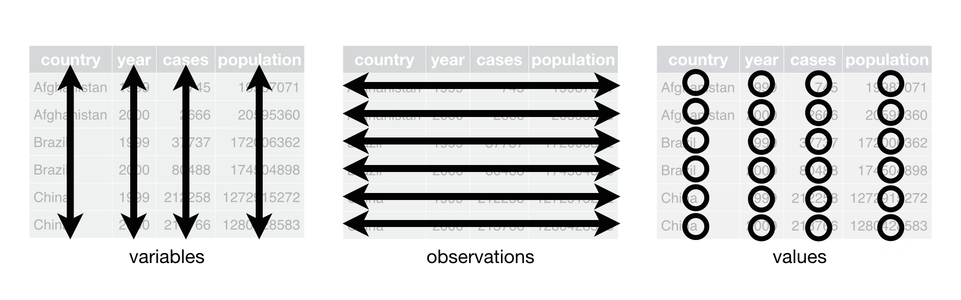
Usually data are untidy in only one way. However, if you are unlucky, they are really untidy and thus a pain to work with…

Tidy Data

Are these data tidy?

Sepal.L.W	Petal.L.W	Species
5.1/3.5	1.4/0.2	setosa
4.9/3	1.4/0.2	setosa
4.7/3.2	1.3/0.2	setosa

Sepal.Length	5.1	4.9	4.7	4.6
Sepal.Width	3.5	3.0	3.2	3.1
Petal.Length	1.4	1.4	1.3	1.5
Petal.Width	0.2	0.2	0.2	0.2
Species	setosa	setosa	setosa	setosa

Tidy Data

Are these data tidy?

Sepal.Length	Sepal.Width	Petal.Length	Petal.Width	Species
5.1	3.5	1.4	0.2	setosa
4.9	3.0	1.4	0.2	setosa
4.7	3.2	1.3	0.2	setosa

Species	variable	value
setosa	Sepal.Length	5.1
setosa	Sepal.Length	4.9
setosa	Sepal.Length	4.7

Tidying Data with `pivot_longer`

If some of your column names should be values of a variable, use pivot_longer (which modernizes the legacy gather):

jewels2 |> head(n = 5)

# A tibble: 5 × 3
  cut     `2008` `2009`
  <ord>    <int>  <dbl>
1 Ideal      326    329
2 Premium    326    329
3 Good       327    330
4 Premium    334    337
5 Good       335    338

jewels2 |> 
  pivot_longer(cols = c(`2008`, `2009`), names_to = 'year', values_to = 'price') |>
  head(n = 5)

# A tibble: 5 × 3
  cut     year  price
  <ord>   <chr> <dbl>
1 Ideal   2008    326
2 Ideal   2009    329
3 Premium 2008    326
4 Premium 2009    329
5 Good    2008    327

Tidying Data with `pivot_wider`

If some of your observations are scattered across many rows, use pivot_wider (which modernizes the legacy spread):

jewels3

# A tibble: 9 × 5
  cut     price clarity dimension measurement
  <ord>   <int> <ord>   <chr>           <dbl>
1 Ideal     326 SI2     x                3.95
2 Premium   326 SI1     x                3.89
3 Good      327 VS1     x                4.05
4 Ideal     326 SI2     y                3.98
5 Premium   326 SI1     y                3.84
6 Good      327 VS1     y                4.07
7 Ideal     326 SI2     z                2.43
8 Premium   326 SI1     z                2.31
9 Good      327 VS1     z                2.31

jewels3 |>
  pivot_wider(names_from = dimension, values_from = measurement) |> 
  head(n = 5)

# A tibble: 3 × 6
  cut     price clarity     x     y     z
  <ord>   <int> <ord>   <dbl> <dbl> <dbl>
1 Ideal     326 SI2      3.95  3.98  2.43
2 Premium   326 SI1      3.89  3.84  2.31
3 Good      327 VS1      4.05  4.07  2.31

Tidying Data with `separate`

If some of your columns contain more than one value, use separate_wider_delim – the secure, explicit replacement for legacy separate():

# A tibble: 2 × 4
  cut     price clarity dim           
  <ord>   <int> <ord>   <chr>         
1 Ideal     326 SI2     3.95/3.98/2.43
2 Premium   326 SI1     3.89/3.84/2.31

jewels4 |>
  separate_wider_delim(dim, delim = "/", names = c("x", "y", "z"))

# A tibble: 2 × 6
  cut     price clarity x     y     z    
  <ord>   <int> <ord>   <chr> <chr> <chr>
1 Ideal     326 SI2     3.95  3.98  2.43 
2 Premium   326 SI1     3.89  3.84  2.31

Note

The modern separate_wider_* function family is strict, meaning it will explicitly alert you with an error if rows contain an uneven balance of delimiters!

Handling Mismatches in wider splits

The modern separate_wider_delim() is strict. By default, it will throw an error if the delimiter count is inconsistent across rows. Use too_few and too_many to handle uneven data:

jewels4 |> 
  separate_wider_delim(
    cols = dim, 
    delim = "/", 
    names = c("x", "y", "z"),
    too_few = "align_start",  # Options: "align_start", "align_end", "debug"
    too_many = "drop" # Options: "drop", "merge"
  )

Strict Validation: No more silent misalignments like in the legacy separate().

Debug Mode: Setting too_few = "debug" creates temporary logical columns identifying exactly where and why splits failed.

Tidying Data with `unite`

If some of your columns contain elements that need to be grouped together:

# A tibble: 5 × 7
  cut     price clarity_prefix clarity_suffix     x     y     z
  <ord>   <int> <chr>          <chr>          <dbl> <dbl> <dbl>
1 Ideal     326 SI             2               3.95  3.98  2.43
2 Premium   326 SI             1               3.89  3.84  2.31
3 Good      327 VS             1               4.05  4.07  2.31
4 Premium   334 VS             2               4.2   4.23  2.63
5 Good      335 SI             2               4.34  4.35  2.75

jewels5 |> unite(clarity, clarity_prefix, clarity_suffix, sep='')

# A tibble: 5 × 6
  cut     price clarity     x     y     z
  <ord>   <int> <chr>   <dbl> <dbl> <dbl>
1 Ideal     326 SI2      3.95  3.98  2.43
2 Premium   326 SI1      3.89  3.84  2.31
3 Good      327 VS1      4.05  4.07  2.31
4 Premium   334 VS2      4.2   4.23  2.63
5 Good      335 SI2      4.34  4.35  2.75

Missing Data – the `!is.na()` boilerplate problem

A common pattern in data cleaning:

simple
complex

df |>
  filter(!is.na(x))

df |>
  filter(!is.na(x) & !is.na(y) & !is.na(z))

option 1
option 2

df |> drop_na(x)
df |> drop_na(x, y, z)

less boilerplate
easier to read
explicit intent: remove missing rows

Instead of removing rows, sometimes you want to fill missing values:

df |> mutate(x = coalesce(x, y, z))

This means Take the first non-NA value across these columns.

Completing Missing Values Using `complete`

jewels |> head(n = 10) |> select(cut, clarity, price) |> 
  mutate(continent = sample(c('Aus', 'Eur'), size = 6, replace = T)) -> missing_stones

missing_stones |> complete(cut, continent) |> head(n = 7)

# A tibble: 7 × 4
  cut       continent clarity price
  <ord>     <chr>     <ord>   <int>
1 Fair      Aus       <NA>       NA
2 Fair      Eur       <NA>       NA
3 Good      Aus       VS1       327
4 Good      Eur       SI2       335
5 Very Good Aus       <NA>       NA
6 Very Good Eur       VVS2      336
7 Premium   Aus       SI1       326

Combining Datasets

Often, we need to combine a number of data tables (relational data) to get the full picture of the data. Here different types of joins come to help:

mutating joins that add new variables to data table A based on matching observations (rows) from data table B

filtering joins that filter observations from data table A based on whether they match observations in data table B

set operations that treat observations in A and B as elements of a set.

Let us create two example tibbles that share a key:

key	x
a	A1
b	A2
c	A3
e	A4

key	y
a	B1
b	NA
c	B3
d	B4

The Joins Family — `inner_join`

key	x
a	A1
b	A2
c	A3
e	A4

key	y
a	B1
b	NA
c	B3
d	B4

A |> inner_join(B, by = 'key')
# All non-matching rows are dropped!

# A tibble: 3 × 3
  key   x     y    
  <chr> <chr> <chr>
1 a     A1    B1   
2 b     A2    <NA> 
3 c     A3    B3

The Joins Family — `left_join`

key	x
a	A1
b	A2
c	A3
e	A4

key	y
a	B1
b	NA
c	B3
d	B4

A |> left_join(B, by = 'key')

# A tibble: 4 × 3
  key   x     y    
  <chr> <chr> <chr>
1 a     A1    B1   
2 b     A2    <NA> 
3 c     A3    B3   
4 e     A4    <NA>

The Joins Family — `right_join`

key	x
a	A1
b	A2
c	A3
e	A4

key	y
a	B1
b	NA
c	B3
d	B4

A |> right_join(B, by = 'key')

# A tibble: 4 × 3
  key   x     y    
  <chr> <chr> <chr>
1 a     A1    B1   
2 b     A2    <NA> 
3 c     A3    B3   
4 d     <NA>  B4

The Joins Family — `full_join`

key	x
a	A1
b	A2
c	A3
e	A4

key	y
a	B1
b	NA
c	B3
d	B4

A |> full_join(B, by = 'key')

# A tibble: 5 × 3
  key   x     y    
  <chr> <chr> <chr>
1 a     A1    B1   
2 b     A2    <NA> 
3 c     A3    B3   
4 e     A4    <NA> 
5 d     <NA>  B4

Some Other Friends

stringr for string manipulation and regular expressions
forcats for working with factors
lubridate for working with dates (now in the tidyverse core)

Thank you!

Questions?

2026 • SciLifeLab • NBIS • RaukR

Tidy work in Tidyverse

Learning Outcomes

Tidyverse — what is it all about?

?(Tidyverse OR !Tidyverse)

Typical Tidyverse Workflow

Introduction to Pipes or Let My Data Flow 🌊

Introduction to Pipes

Other Types of Pipes — %T>%

Other Types of Pipes — %T>%

Other Types of magrittr Pipes — %$%

Other Types of magrittr Pipes — %<>%

Native R pipe

Placeholders in magrittr Pipes

Placeholders for nested expressions

Placeholders – unary functions

Time to do Lab 1.1

Tibbles

Convert data.frame to tibble

Tibbles from scratch with tibble

More on Tibbles

Tibble printing options

Subsetting Tibbles

Partial Matching

Non-existing Columns

Time to do Lab 1.2

Loading Data

Loading Data

Under the Hood – parse_* Functions

Parsing Strings

Parsing Factors

Other Parsing Functions

Writing to a File

Time to do Lab 1.3

Basic Data Transformations with dplyr

Picking Observations using filter()

Floating point and tidyverse

Rearranging Observations using arrange()

Selecting Variables with select()

Renaming variables

Bring columns to front

Create/alter new Variables with mutate

Conditional mutate

Create/alter new Variables with transmute 🧙‍♂️

Group and Summarize

More on (un-)grouping

Other data manipulation tips

The Concept of Tidy Data

Tidy Data

Tidy Data

Tidying Data with pivot_longer

Tidying Data with pivot_wider

Tidying Data with separate

Handling Mismatches in wider splits

Tidying Data with unite

Missing Data – the !is.na() boilerplate problem

Completing Missing Values Using complete

Combining Datasets

The Joins Family — inner_join

The Joins Family — left_join

The Joins Family — right_join

The Joins Family — full_join

Some Other Friends

`?(Tidyverse OR !Tidyverse)`

Other Types of Pipes — `%T>%`

Other Types of Pipes — `%T>%`

Other Types of `magrittr` Pipes — `%$%`

Other Types of `magrittr` Pipes — %<>%

Placeholders in `magrittr` Pipes

Convert `data.frame` to `tibble`

Tibbles from scratch with `tibble`

Under the Hood – `parse_*` Functions

Basic Data Transformations with `dplyr`

Picking Observations using `filter()`

Floating point and `tidyverse`

Rearranging Observations using `arrange()`

Selecting Variables with `select()`

Create/alter new Variables with `mutate`

Create/alter new Variables with `transmute` 🧙‍♂️

Tidying Data with `pivot_longer`

Tidying Data with `pivot_wider`

Tidying Data with `separate`

Tidying Data with `unite`

Missing Data – the `!is.na()` boilerplate problem

Completing Missing Values Using `complete`

The Joins Family — `inner_join`

The Joins Family — `left_join`

The Joins Family — `right_join`

The Joins Family — `full_join`