Statistical Learning
RaukR 2026 • Data Science With R
20-Aug-2026
R and bioinformatics - the Bioconductor project
- “The mission of the Bioconductor project is to develop, support, and disseminate free open source software that facilitates rigorous and reproducible analysis of data from current and emerging biological assays. We are dedicated to building a diverse, collaborative, and welcoming community of developers and data scientists.”

- Current release (2.23):
- 2,418 software packages
- 928 AnnotationData packages
- 436 ExperimentData packages
- 28 Workflows
- 8 books

EuroBioc 2026 Turku, Finland (June 3-5)

25 years of Bioconductor

Conferences
- BioC – Aug 10-12 in Seattle
- BiocAsia – next one in Melbourne, Australia Nov 19-20, 2026
- EuroBioC – next one in Basel, Switzerland Sept 8-10, 2027 (pre-conf 6-7)
 Caroline Uhler
 Davide Risso
 Mireia Ramos-Rodríguez
 Luca Giorgetti
 Daria Lazic
- Zulip channel open to everyone
R and statistics

Statistical methods are developed to be used in the real world!
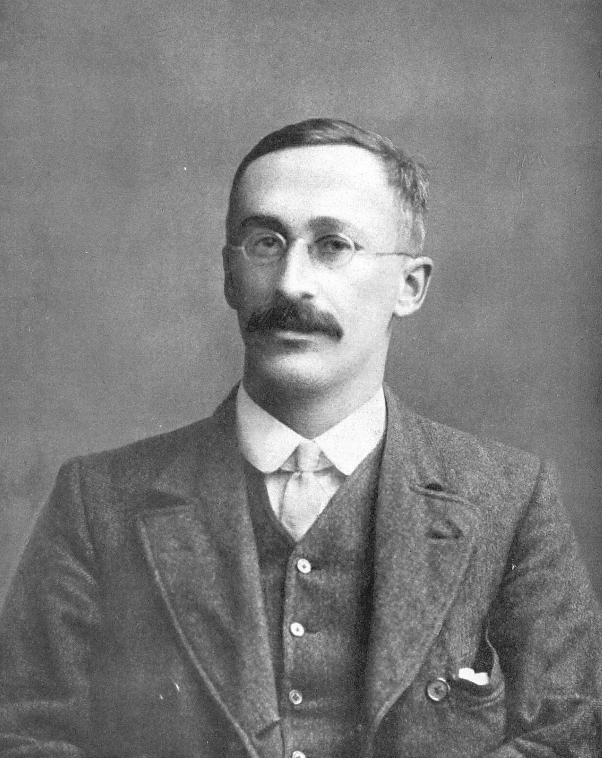
- William Sealy Gosset worked as a chemist and brewer at Guinness Brewery in Dublin in the early 1900s.
- Used pen name Student because Guinness prohibited employees from publishing research under their own names.
- Guiness wanted to improve barley varieties and beer quality.
- Experiments with small sample sizes. The population variance is unknown and must be estimated.
- Student’s t-distribution and test of statistical significance.
Early examples of learning something about the world
- Eratosthenes: ancient Greek philosopher, scholar, mathematician, geographer, poet, astronomer and music theorist.
- Estimating the circumference of the earth in 240 BC.
- Assumptions:
- earth is round
- sun is so far the rays coming from there are parallel
- distance between Alexandria and Syene is known
- \(\frac{7.2^\circ}{360^\circ}=\frac{ditance \ between \ Alexandria \ and \ Aswan}{Earth's \ circumference}\)
- His estimate: approximately 40,338 km (25,065 mi)
- Today’s number (around the equator): 40,075.017 km (24,901.461 mi)

Data science today


- Nowadays, skill set:
- programming
- statistics
- data visualization
- creativity
- data exploration and going hunting for “problems”
- understanding the data and data generation process
- formulating a question and then finding the right method to answer it
- communication in an interdisciplinary world
Hypothesis generation
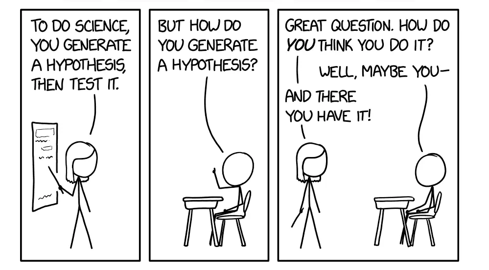
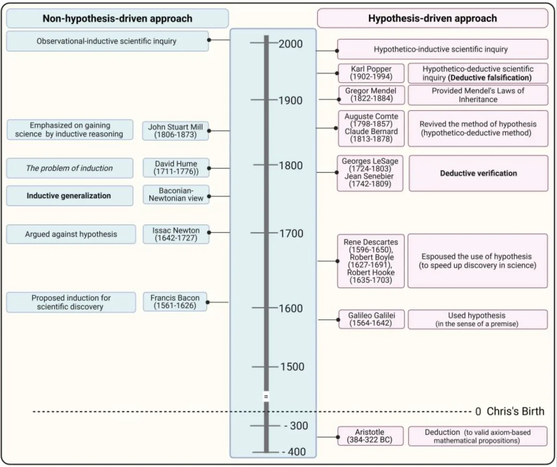
- Formulate a hypothesis -> collect data -> test
- Collect data -> explore -> generate hypothesis
- Explore -> new data -> confirm
- Exploration vs confirmation
Statistical learning
“Statistical learning refers to a set of tools for making sense of complex datasets” – An Introduction to Statistical Learning by James, Witten, Hastie and Tibshirani
Many of these methods were developed long before we had computers, and they are incredibly useful today.
No single methods will perform well or be appropriate for all data set. It is therefore important to understand how these tools work, when to use them and how to interpret the results.
“We are drowning in information and starving for knowledge” – Rutherford D. Roger as quoted in Elements of Statistical Learning
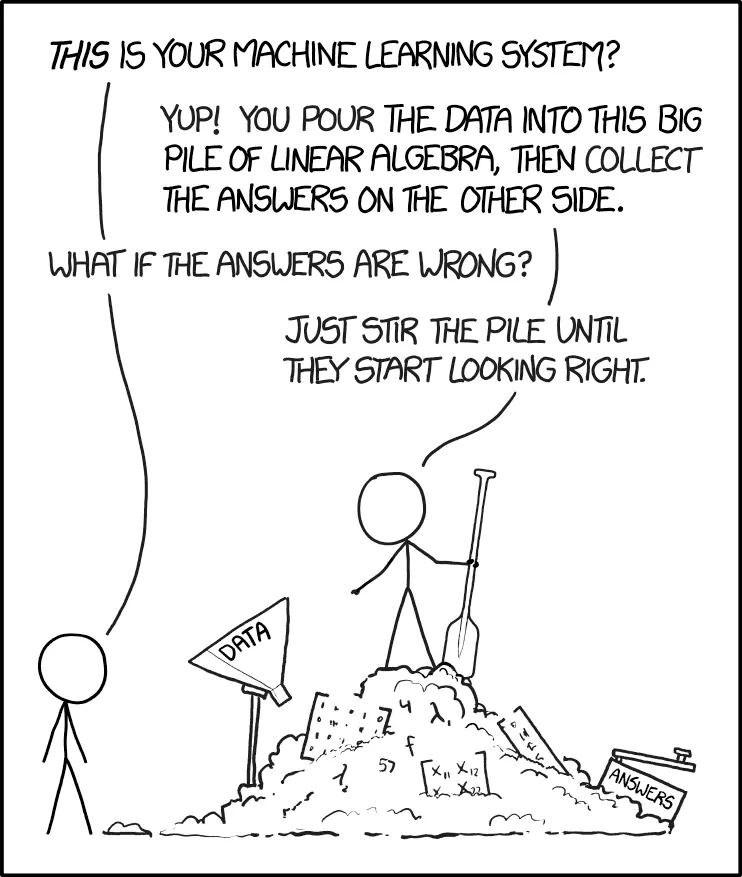
Supervised vs unsupervised learning
Suppose we have measurements for \(p\) variables \(x_1, x_2 ... x_p\) and their associated variable \(y\) and wish to say something about how \(x_1, x_2 ... x_p\) explain or relate to \(y\). An example is prediction or classification.
\(y \sim f(x)\)

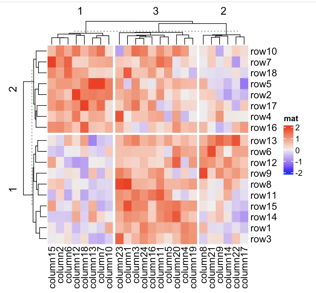
- Suppose we only have measurements for variables \(x_1, x_2 ... x_p\) and wish to learn the relationships between them. An example method is clustering.
Prediction
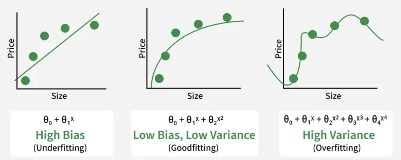
Training data vs test data
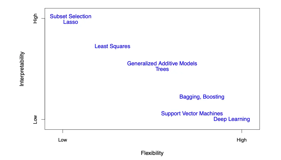
Trade off between prediction accuracy and model interpretability
- Training data: to estimate the model parameters and tune the model.
- Test data: evaluate the model.
- Do you think we can mix both or use the training data to test?
- Our aim here is to use the model on new data and not to explain the data we already have.
- Overfitting – Should we be skeptical when someone claims 100% prediction accuracy with their model?
Inference
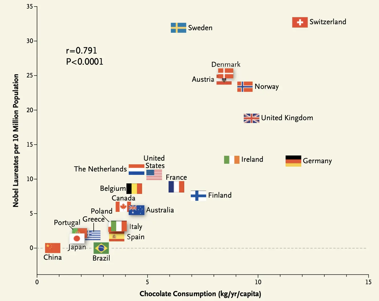
- Which \(x\) variables are associated with the variable \(y\)?
- Can we learn or day something about this relationship?
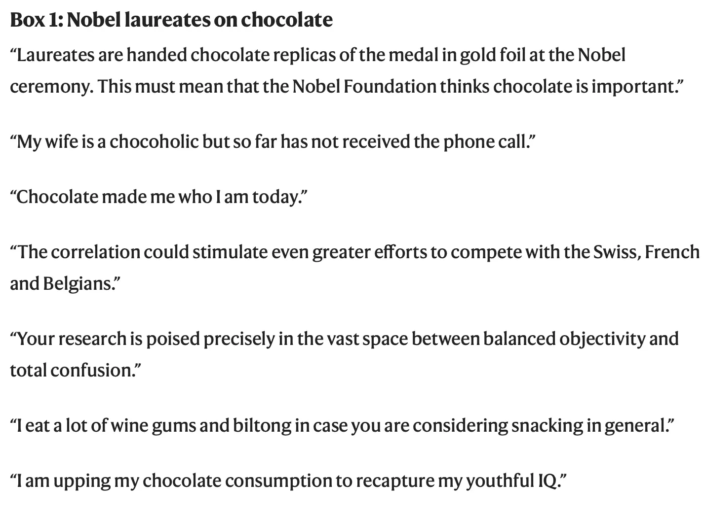
- Suppose we saw the data below, can we use a model to learn the nature of the relationship between the number of Nobel prizes and chocolate consumption?
Choosing the right model
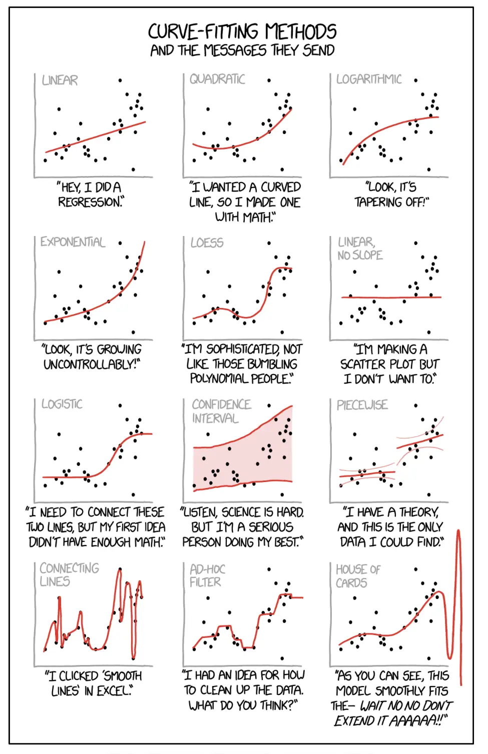
- Do we have prior information about the data?
- Data generation process?
- Expected distributions (e.g. count data)?
- Missing values, missing at random?
- Do we have enough data points?
- Are we trying to learn something about the relationship between our variables or to have a model that we can use to predict outcomes for future data sets?
Why care about linear approaches?
Having a good understanding of linear models is essential for understanding non-linear ones. Many of the latter are generalizations of the linear methods.
Powerful in their interpretability and in their flexibility
If we are interested in inference then retaining interpretability is key
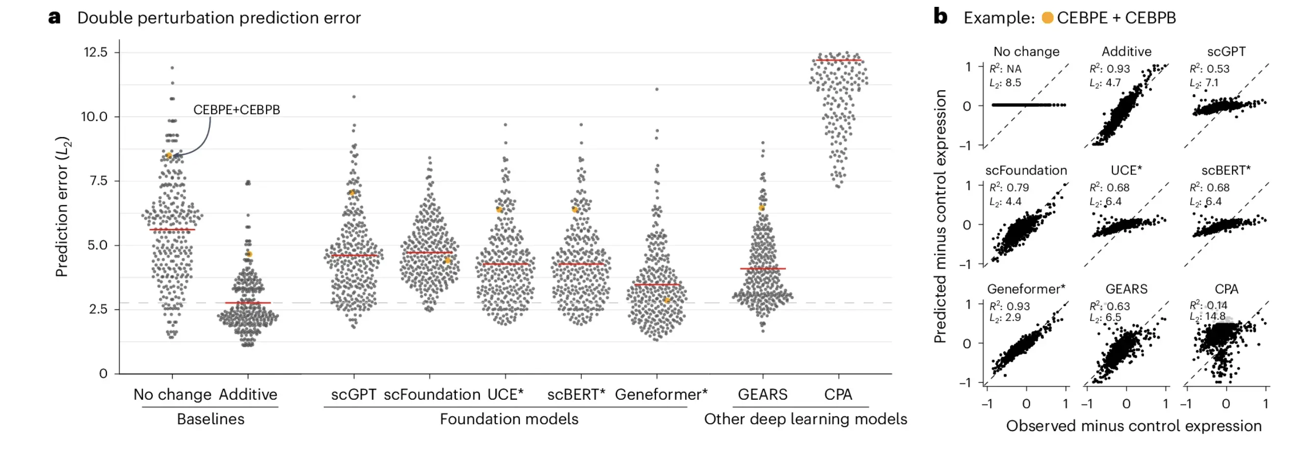
Simple linear regression
learn the association between a single predictor \(x\) and a quantitative response \(y\).
assumes an approximately linear relationship between \(x\) and \(y\).
\[y = \beta_0 + \beta_1x + \epsilon\]
- The error term \(\epsilon\) captures the noise or lack of fit to the linear equation.
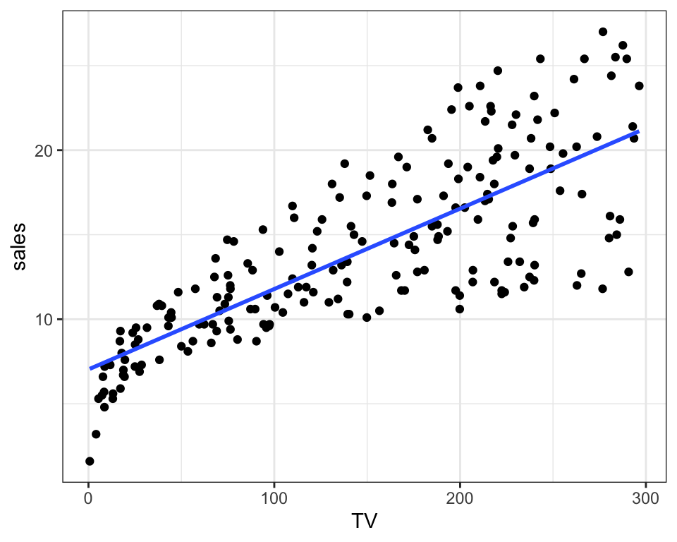
- What do \(\beta_0\) and \(\beta_1\) capture?
- How do we find the best fit?
Least squares
- \(y = \beta_0 + \beta_1x + \epsilon\)
- \(\hat{y_i}=\beta_0 + \beta_1x_i\)
- \(e_i=y_i-\hat{y_i}\)
The residual sum of squares (RSS) is defined as \(RSS=\sum_{i=1}^Ne_i^2\)
We want to choose beta estimates which minimize the RSS. This is the least squares method.
Least squares was developed at the beginning of the 19th century (earliest form of linear regression), with applications in astronomy.
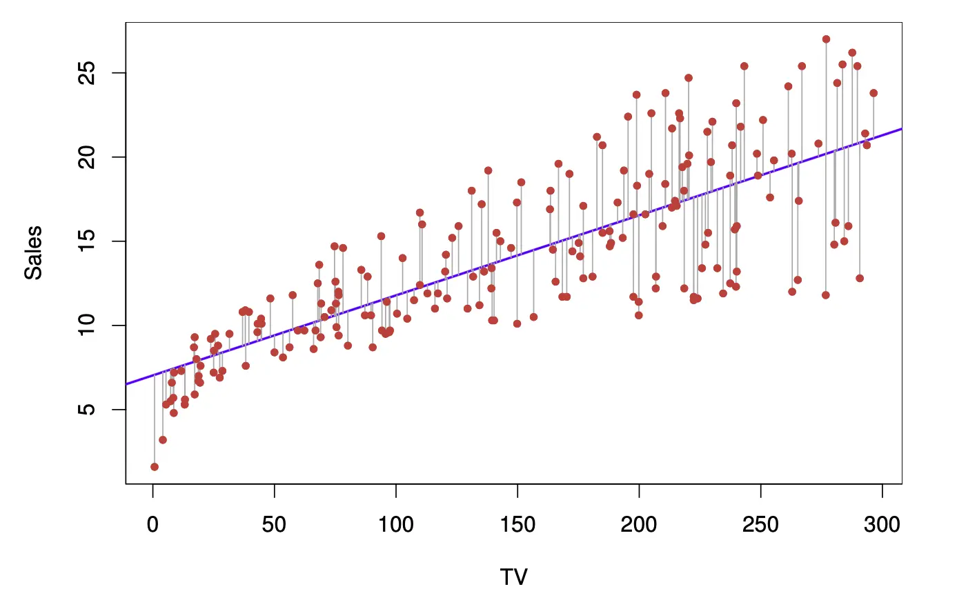
Can you think of another way?
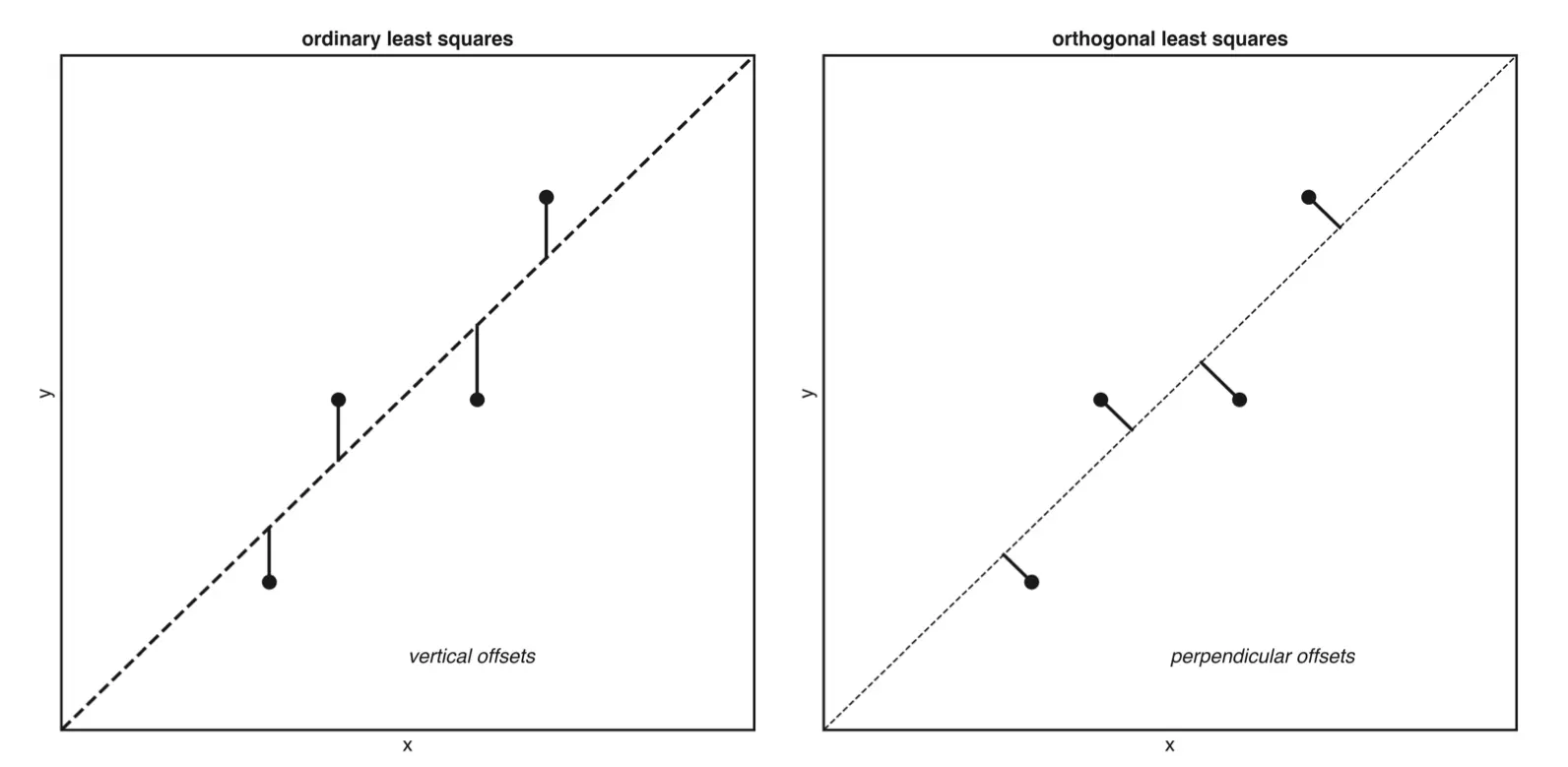
- Given \(x\), how far is the prediction off \(y\)?
- What line lies closest to the cloud of points regardless of which axis is \(x\) or \(y\)
- Which would you pick?
- Least squares: residuals are capturing unexplained variance and prediction error.
Multiple linear regression
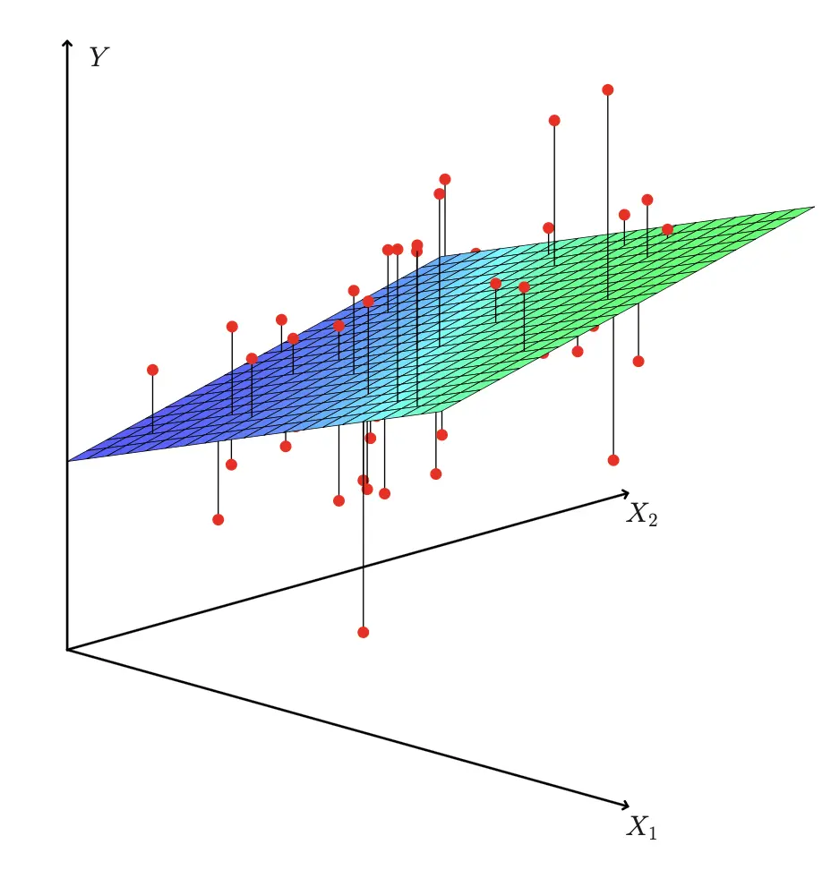
- \(y = \beta_0 + \beta_1x_1 + \beta_2x_2 + ... + \beta_px_p + \epsilon\)
- \(y = \beta.X + \epsilon\)
- Assumptions:
- given x and y values, estimate the coefficients
- linear relationship
- constant variance of residuals (homoscedasticity)
- \(\epsilon \sim N(0, \sigma^2)\)
- independence of observations
- no multicollinearity among predictors
- n >> p
How do we interpret the coefficient values?
Call:
lm(formula = sales ~ TV + radio + newspaper, data = advertisingData)

Coefficients:
(Intercept)           TV        radio    newspaper
   2.938889     0.045765     0.188530    -0.001037
\(y = \beta_0 + \beta_1x_1 + \beta_2x_2 + ... + \beta_px_p + \epsilon\)
Evaluating the quality of the linear fit
- Residual standard error \(RSE=\sqrt{\frac{1}{N-p-1}RSS}\)
- Roughly represents the average amount of deviation from the fitted line.
- The size of the RSE value will reflect how poorly the model fits the data.
- Measured in units of \(y\).
- \(R^2=\frac{TSS-RSS}{TSS}\) where \(TSS=\sum(y_i-\bar{y})^2\).
- RSS can be thought of as measuring the variability that is left unexplained after doing the regression.
- The \(R^2\) value thus reflects the proportion of variability in \(y\) that can be explained using \(x\) by performing the regression.
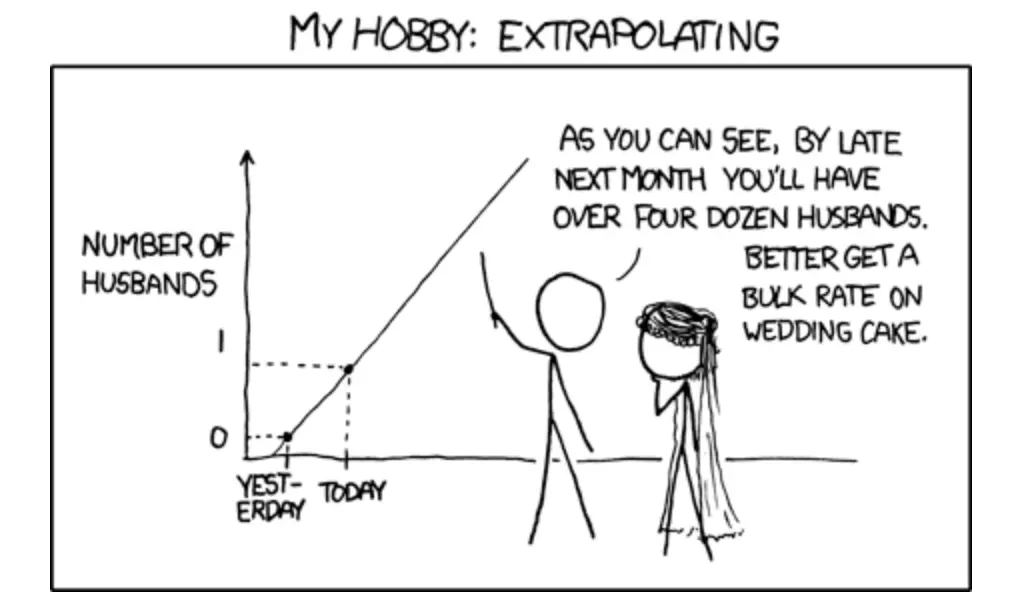
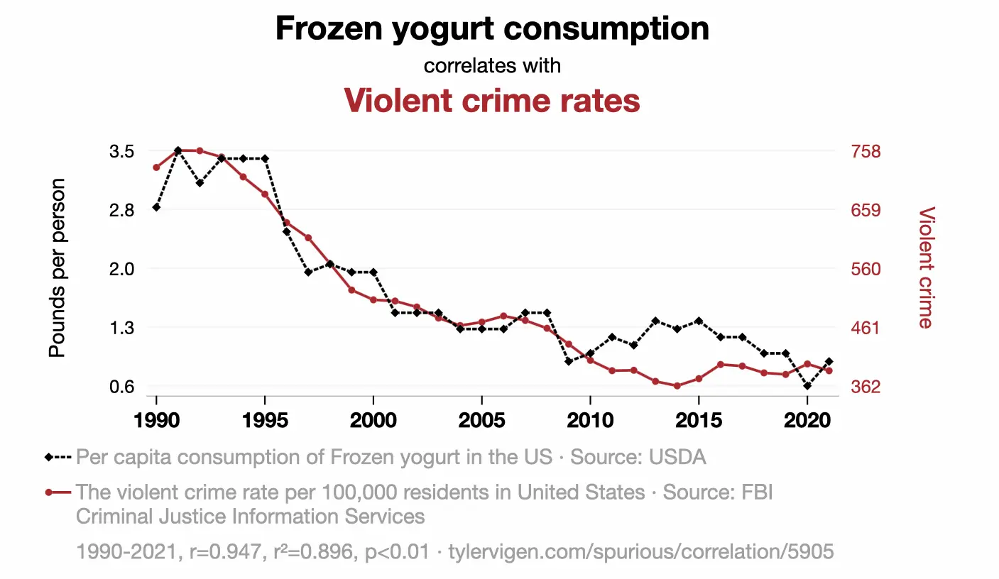
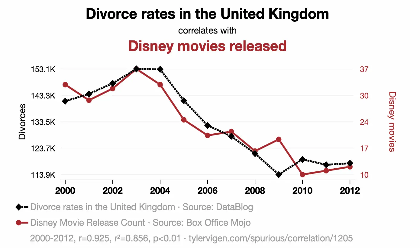
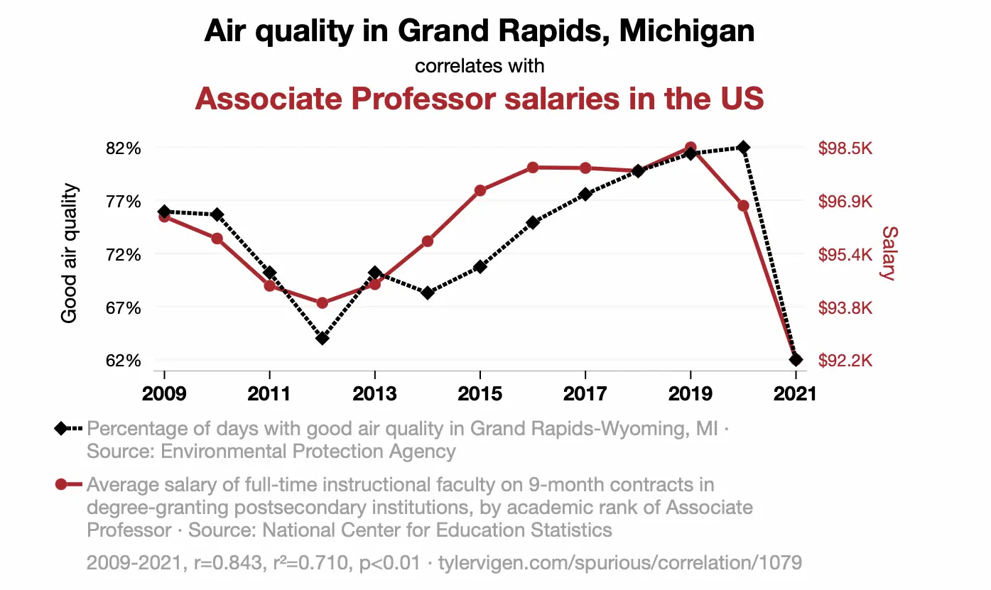
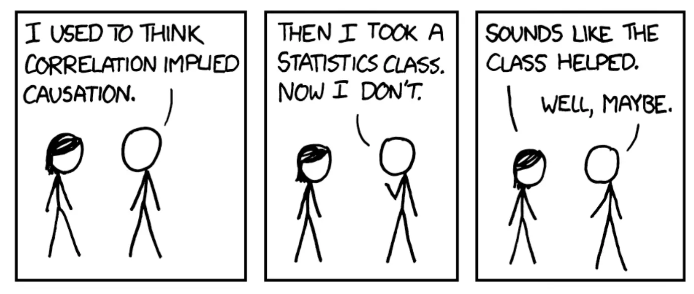
Correlation is not causation
Outliers
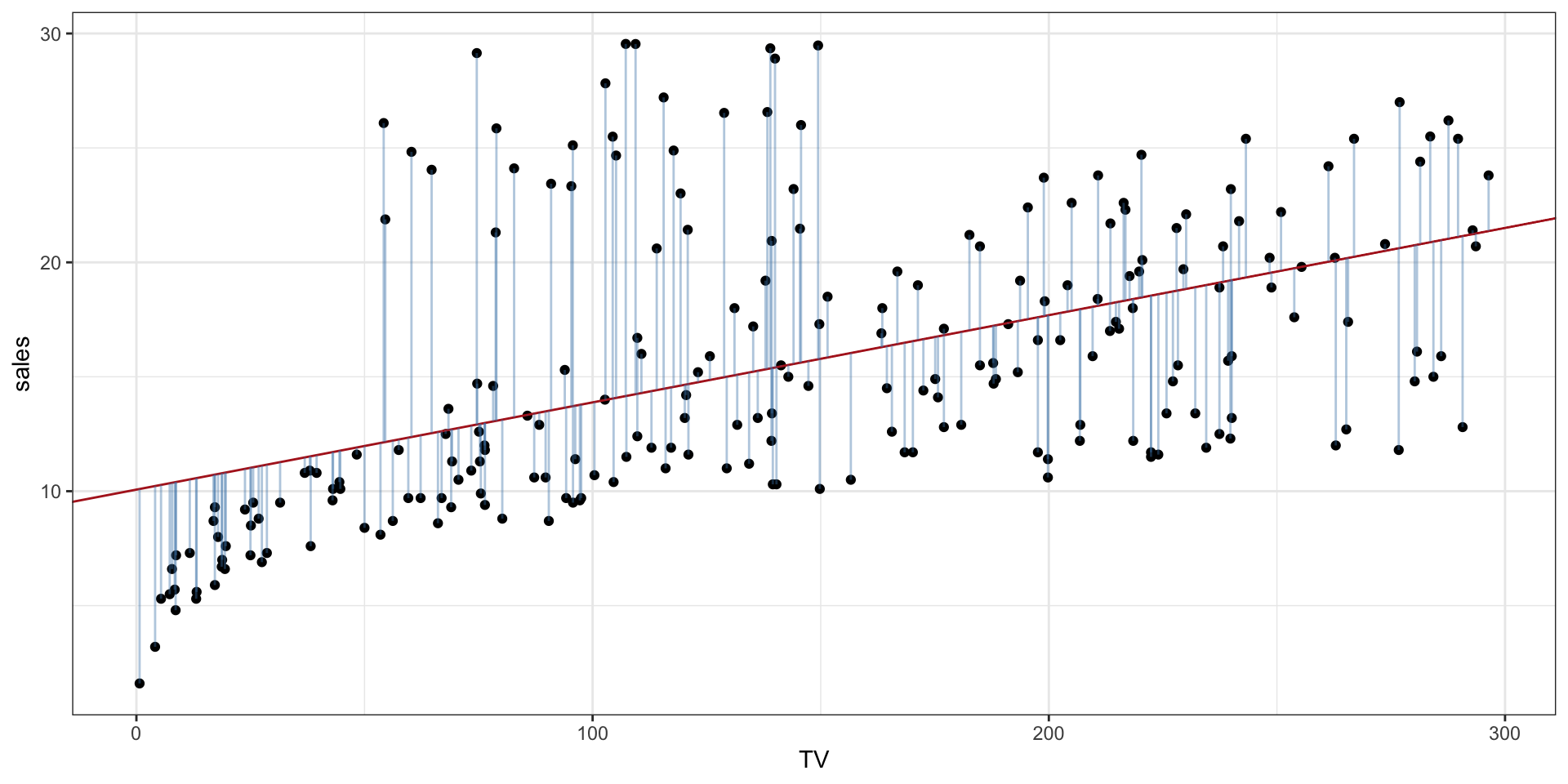
- What is an outlier?
- Why do they arise?
- What do you do with them?
- Can the linear fit be impacted by outliers and when?
- What can you say about the fit and residuals?
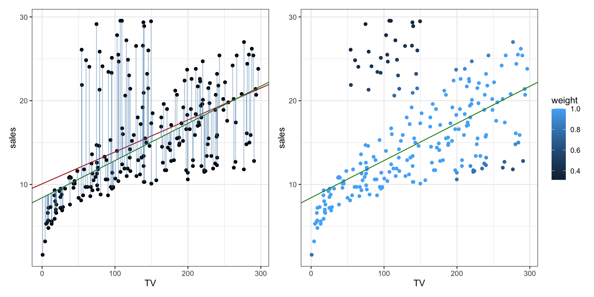
Robust regression
\(RSS=\sum_{i=1}^Ne_i^2\)
Data varies
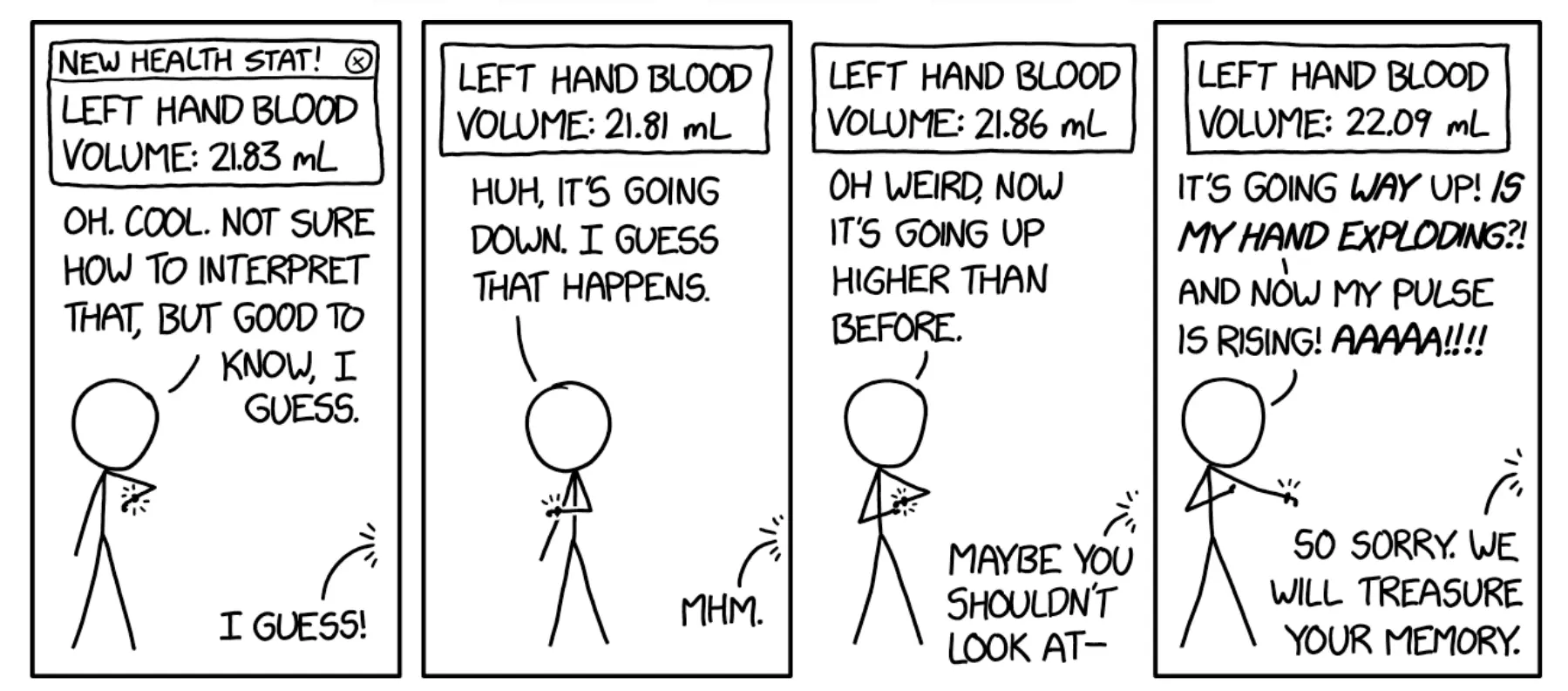
- We draw samples from a population and sample size matters. Is it representative?
- How strong is the signal. How easily is it detected and how much variance does it explain in the data?
- Something to be said for good quality data sets.
Shrinkage methods: ridge
\[ \hat{\beta}=\min\limits_{\beta}\{\sum_{i=1}^N (y_i - \beta_0 - \sum_{j=1}^px_{ij}\beta_j)^2 + \lambda \sum_{j=1}^p\beta_j^2 \} \]
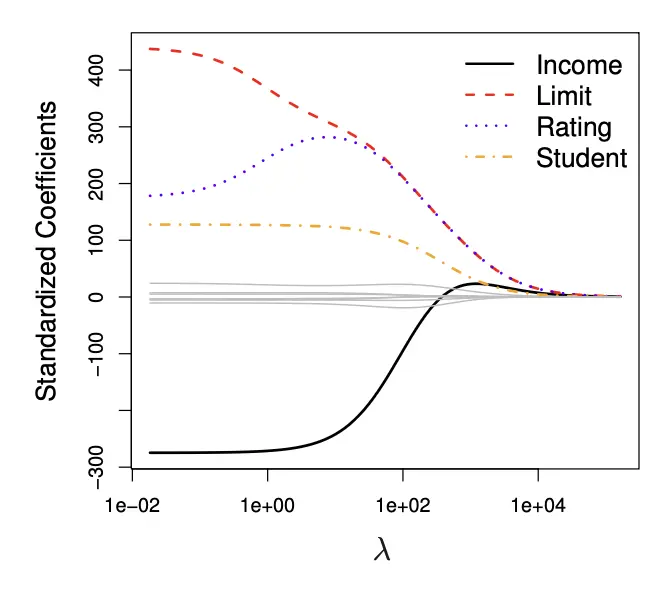
- What is happening to the total sum in the above equation?
- Where are we penalizing more harshly?
- What \(\lambda\) would you choose?
k-fold cross validation
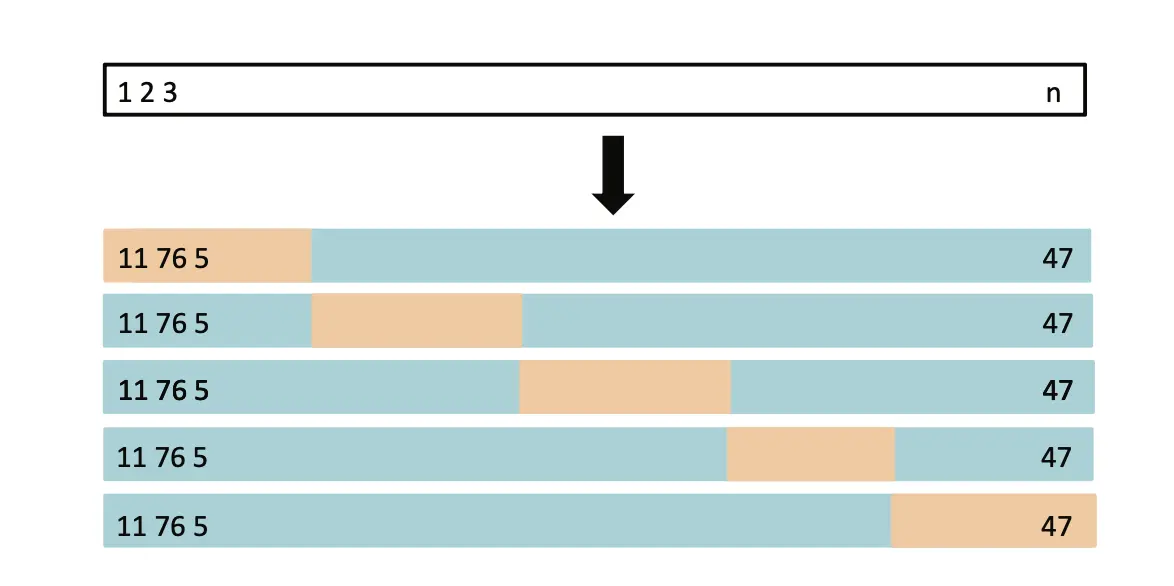
- For each \(\lambda\), train on k-1 folds and test on kth fold.
- Compute prediction error and average the k prediction errors.
- Repeat for each \(\lambda\).
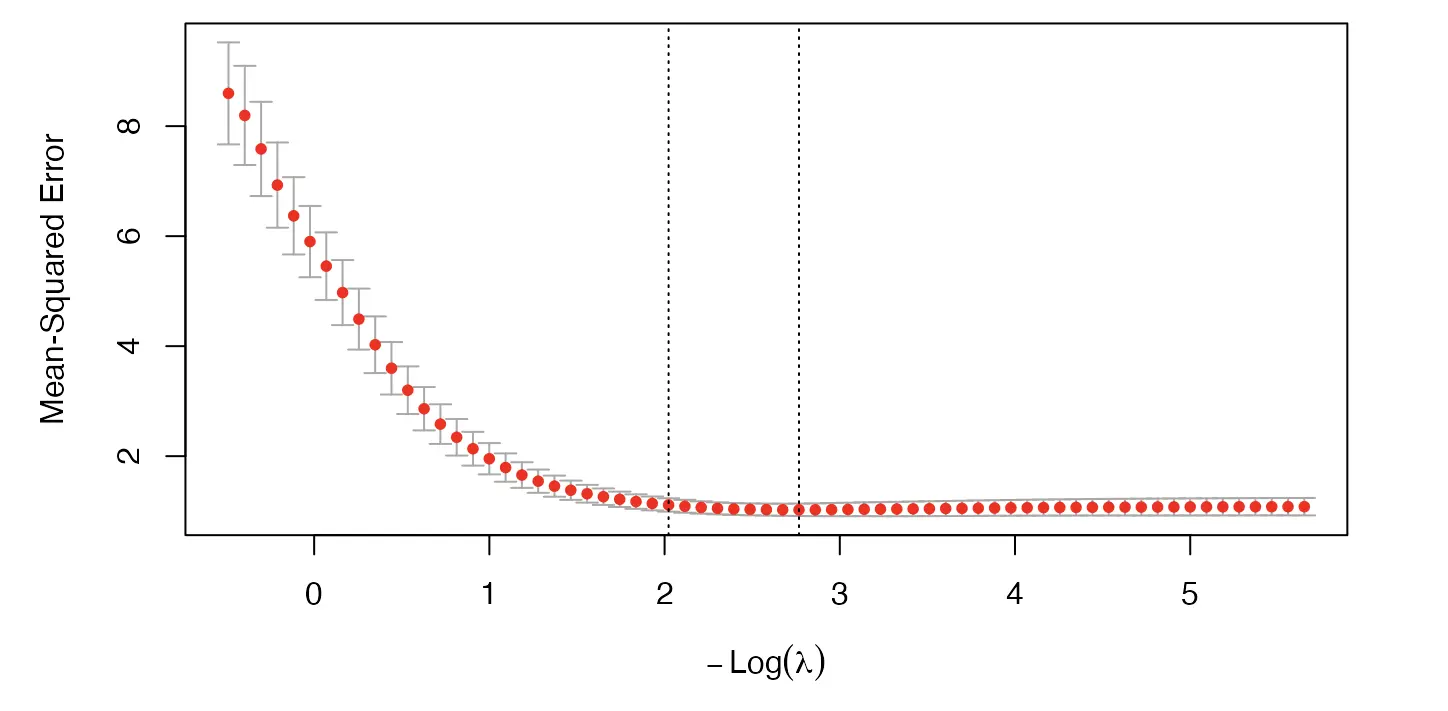
glmnet

[1] 39.65627
[1] 63.144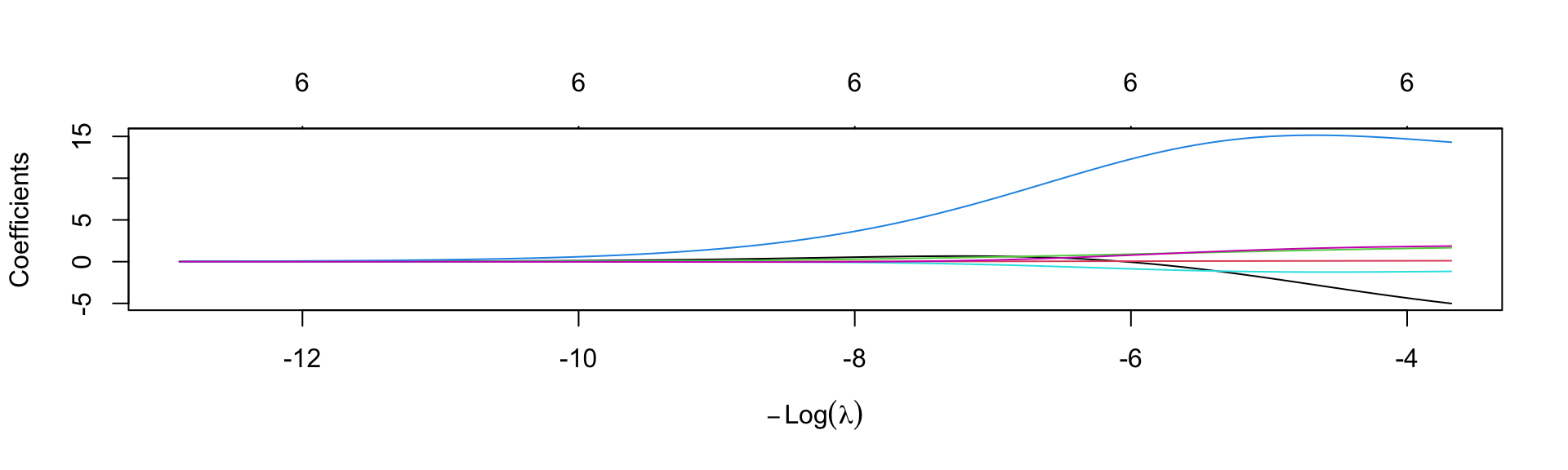
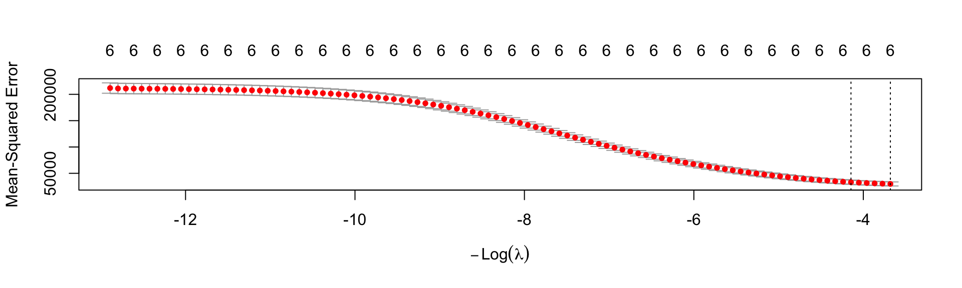
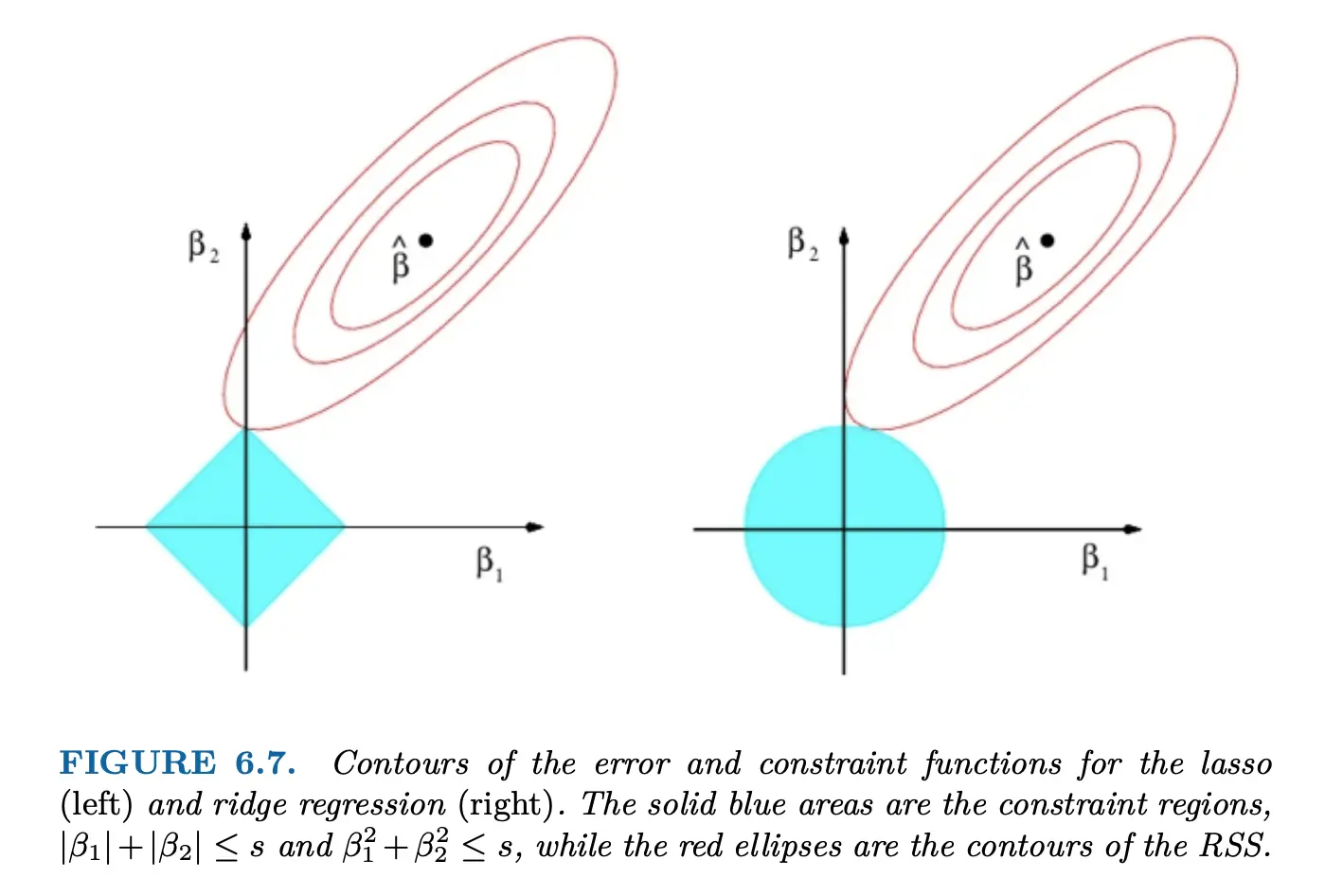
Shrinkage methods: lasso
\[ \hat{\beta}=\min\limits_{\beta}\{\frac{1}{2}\sum_{i=1}^N (y_i - \beta_0 - \sum_{j=1}^px_{ij}\beta_j)^2 + \lambda \sum_{j=1}^p|\beta_j| \} \]
[1] 0.7784687
[1] 15.28166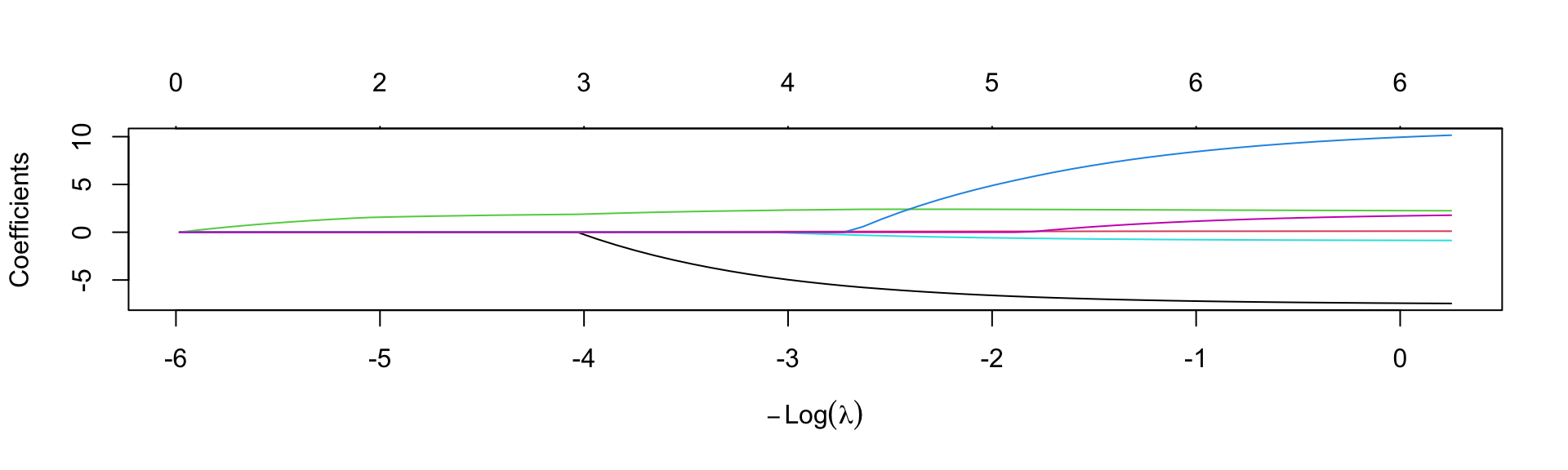
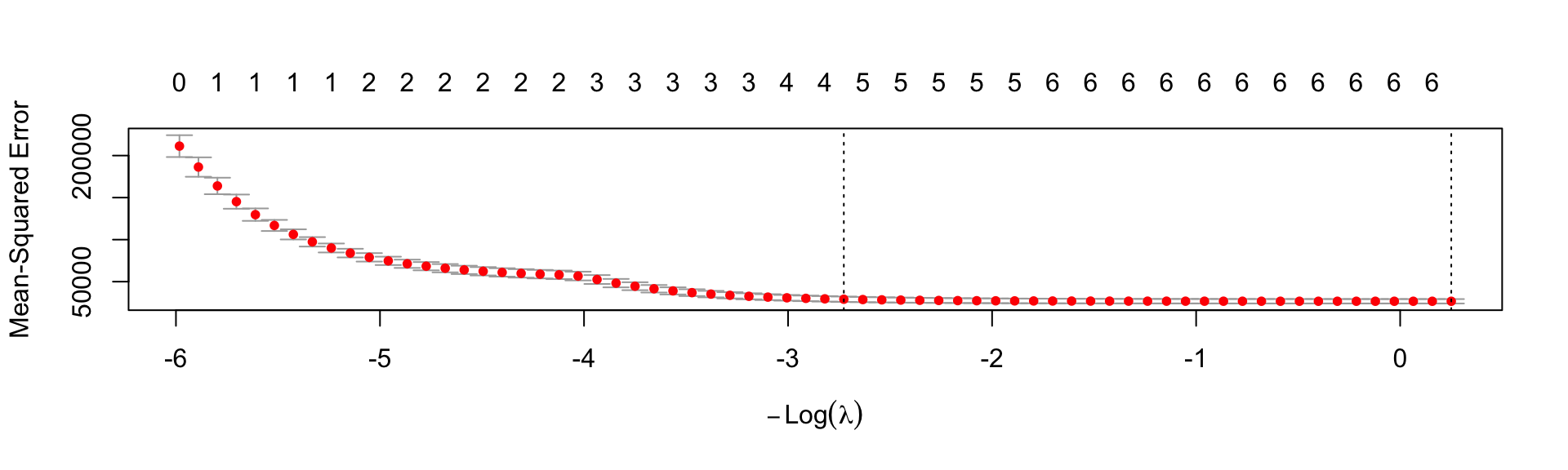
Variable selection with the lasso
- When would we want to make use of such a method?
What do you think the method does when 2 predictors \(x_1\) and \(x_2\) are highly correlated to each other?
Is this problematic?
Collinearity within the predictor matrix:
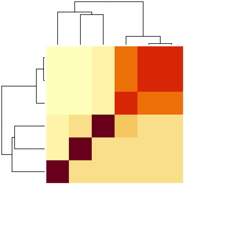
Illustration of the bias-variance trade-off
Stability selection
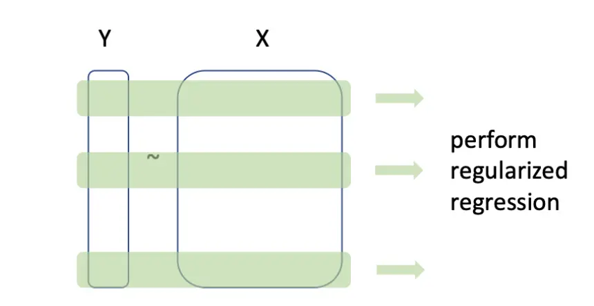
- Can be used when p > N.
- We speak of selection probability values for predictors instead of beta coefficient values.
- How is this calculated with lasso stability selection. If predictor \(x_1\) has a non-zero beta coefficient 80 times and we subset 100 times to do a regression what is its selection probability? Do you think this is high?
\[ \hat{\beta}=\min\limits_{\beta} (||y-X\beta||_2^2 + \lambda \sum_{j=1}^p\frac{|\beta_j|}{W_j} ) \]
- Randomized lasso stability selection.
- Weakness term is between 0 and 1.
- What do you think the effect of the weakness parameter is?
- The randomized lasso changes the penalty λ to a randomly chosen value in the range [λ, λ/weakness].
Stability paths
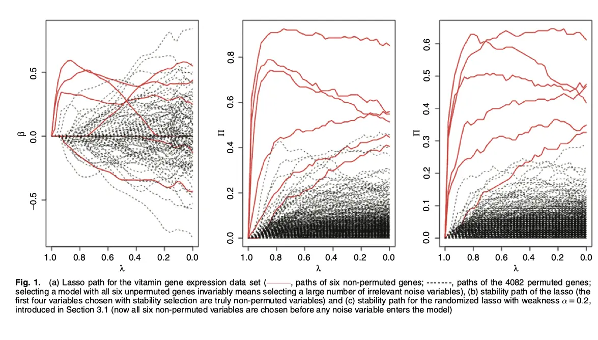
Selecting true predictors
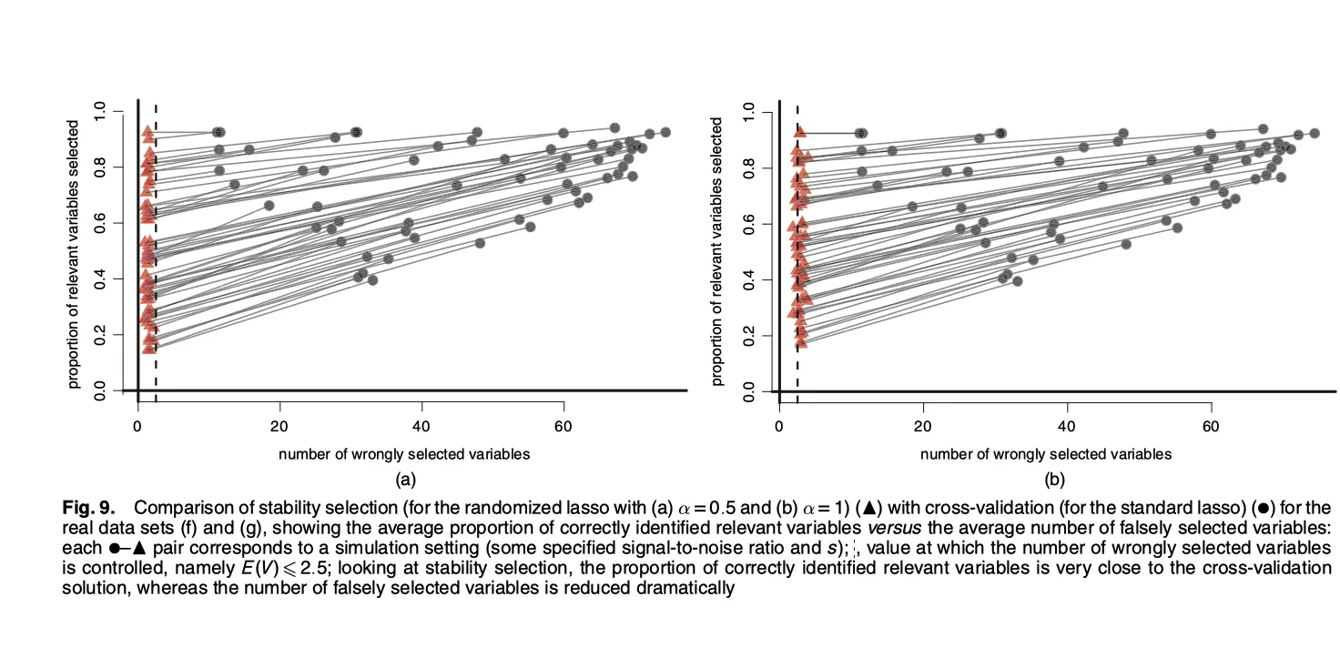
- Regularization with stability selection is rather conservative in practice.
- We need to specify 2 of: probability cutoff, upper bound on PFER, number of selected variables q
- Not slecting a predictor is also a result and telling. Can you think of an example where this could happen?
What about correlated predictors?
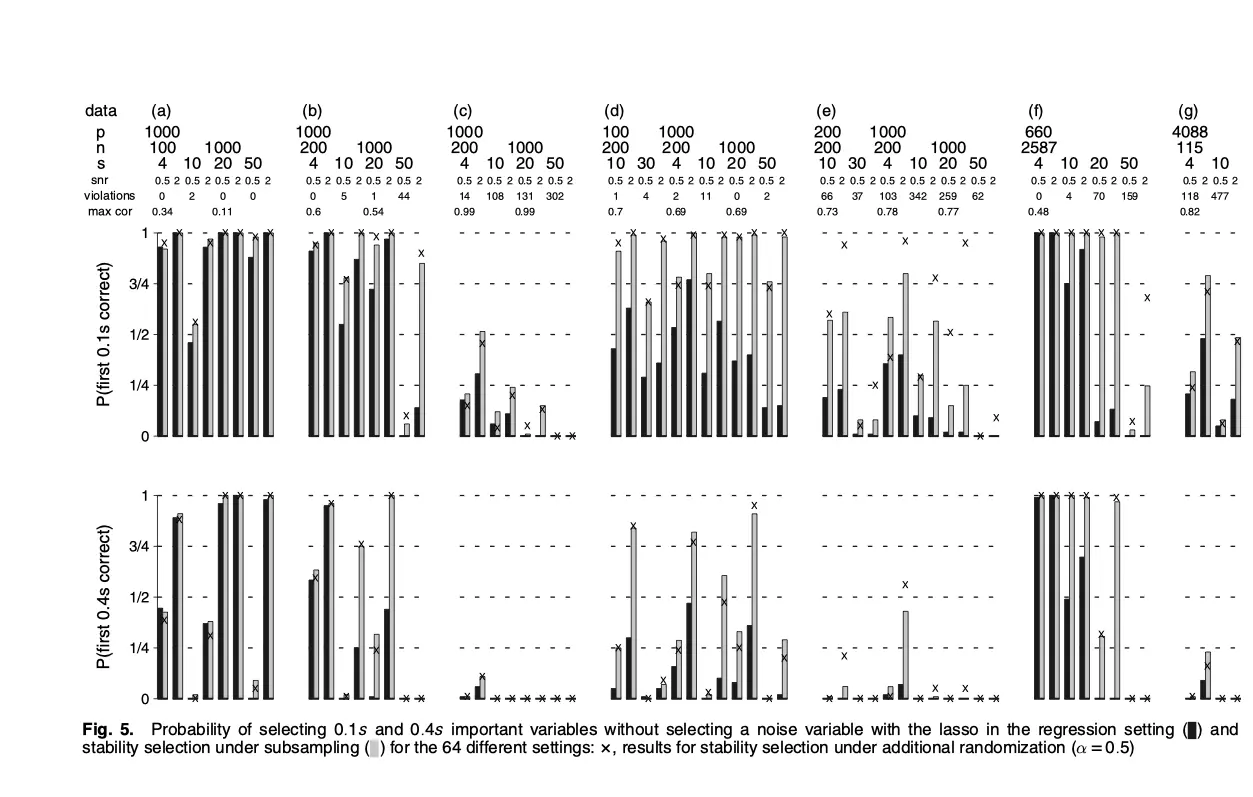
- What did we say about correlated predictors?
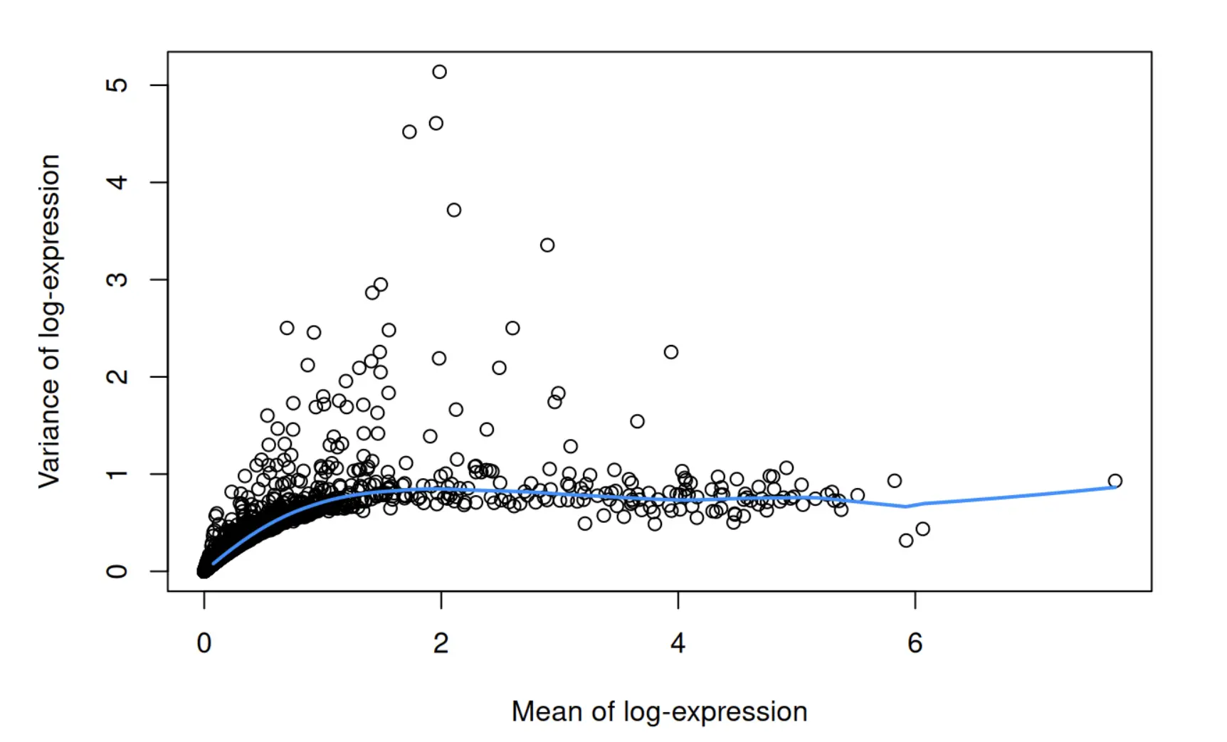
Loess
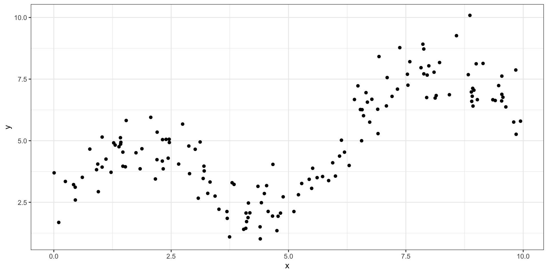
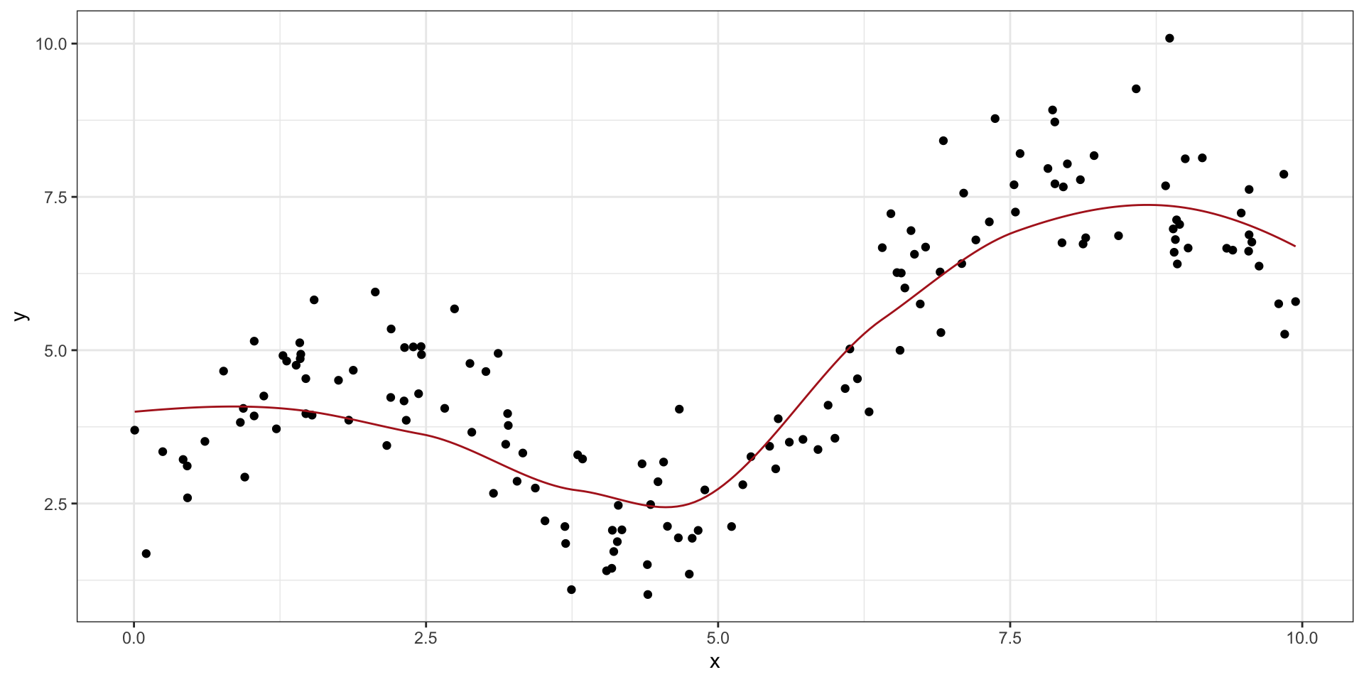
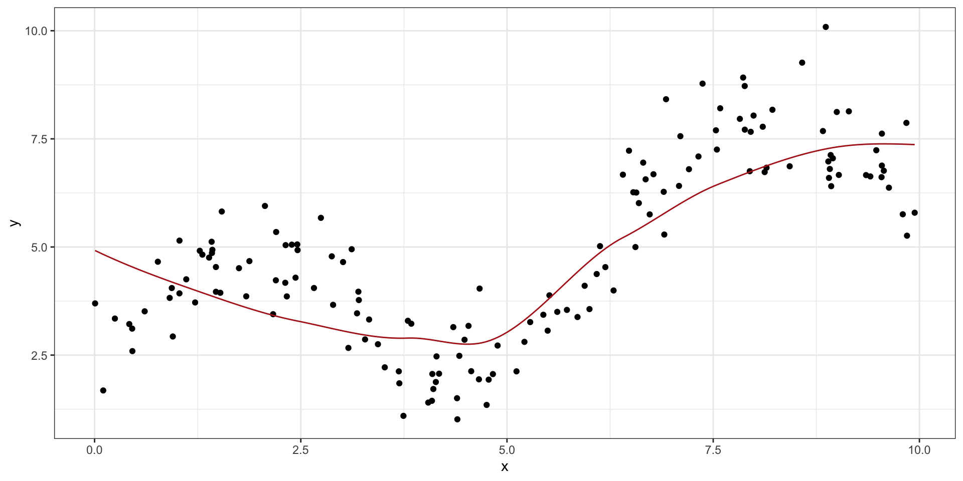
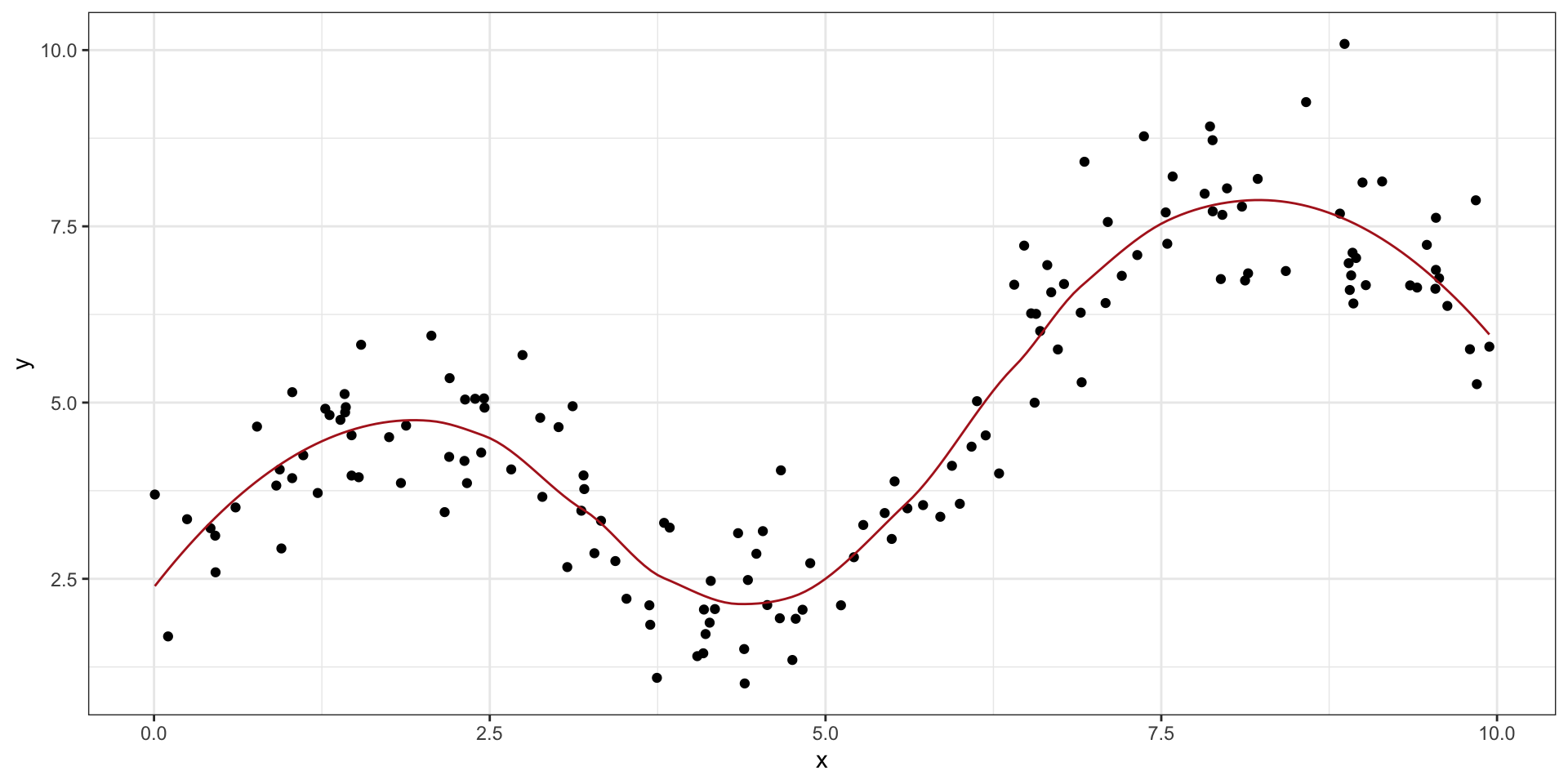
GC bias trends in ATAC-seq/ChIP-seq data
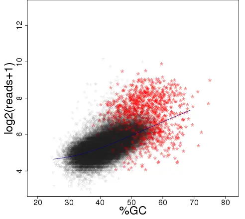
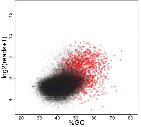
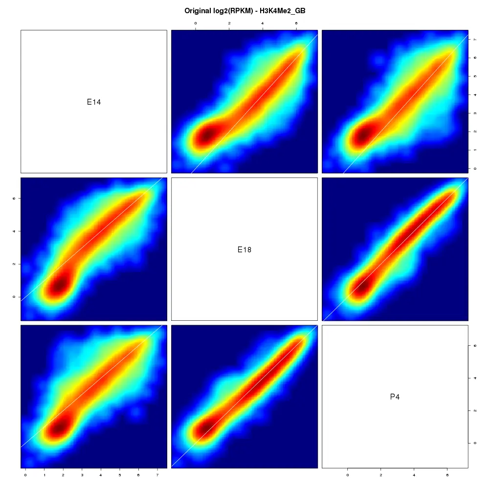
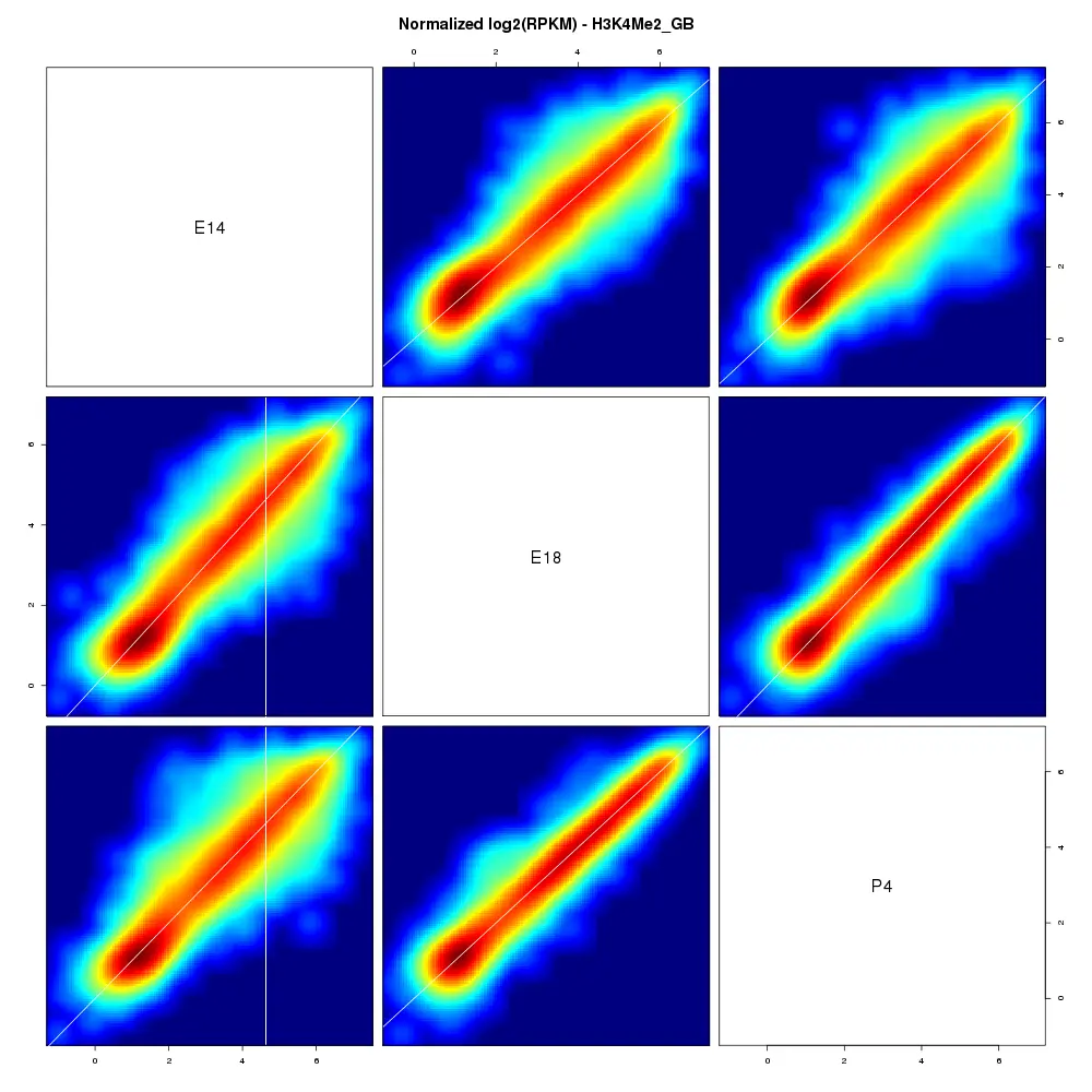
Correcting the trend with limma’s normalizeCyclicLoess()
Experimental design and batch correction
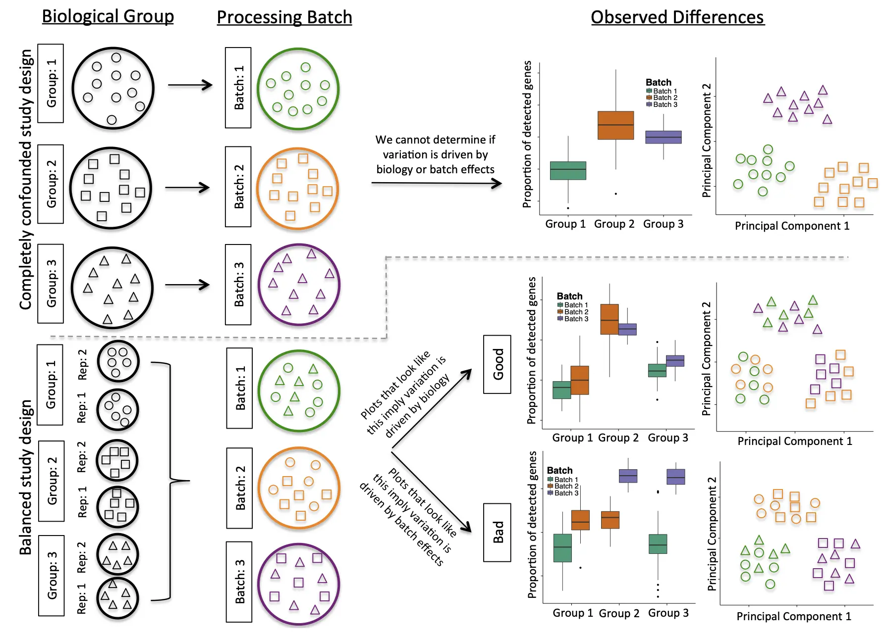
\[y_{observed} = \beta_0 + \beta_{biology}x_{biology} + \beta_{batch}x_{batch} + \epsilon\]
\[y_{corrected} = \beta_0 + \beta_{biology}x_{biology} + \epsilon\]
or
\[y_{corrected} = y_{observed} - \beta_{batch}x_{batch}\]
Gaussian graphical models (GGMs)
- Model statistical relationships between variables using graphs.
- Special algebraic and geometric properties.
- Covariance matrix: covariance between each pair of variables.
- The goal is to estimate the precision matrix (inverse covariance matrix ) which shows the edges in the graph.
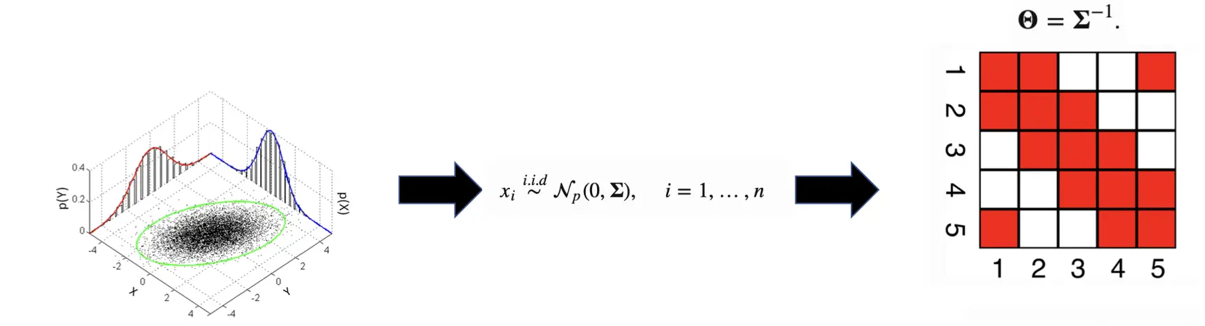
Estimating the (sparse) graph
- Fit lasso on each variable, using all others as predictors.
- Lambda controls sparsity.
- Draw edge with AND/OR rule.
- Edges in the graph reflect meaningful relationships. A missing edge between \(x_1\) and \(x_2\) means those two variables are conditionally independent given all other variables.
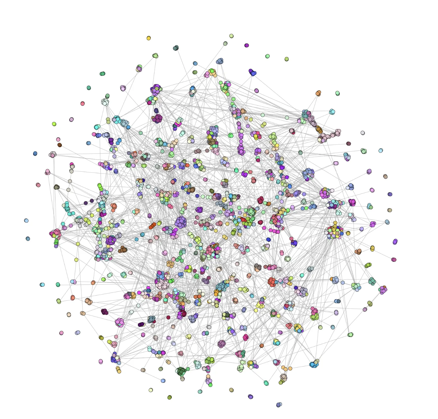
- Example: gene x cell count matrix. We want to learn the gene regulatory network. If necessary, we need to transform the data to look Gaussian to meet the needed assumptions.
glmnetallows you to specify other distribution families that better match the response.
Extra reading/links
- Written by Witten (wxw)
- Nicolei Meinshausen’s website
- Spurious correlations
- Journal of the Royal Statistical Society Series B
- Statistical Ideas that Changed the World
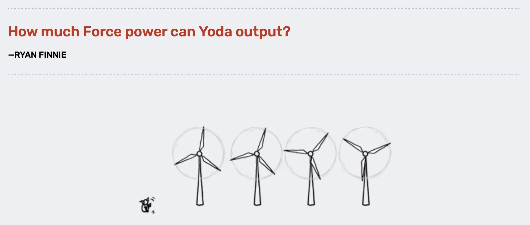
- https://what-if.xkcd.com/archive/
- https://xkcd.com
Resources
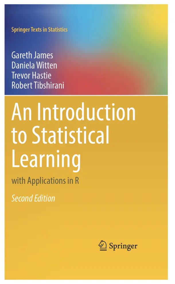
An Introduction to Statistical Learning with applications in R – Gareth James, Daniela Witten, Trevor Hastie and Robert Tibshirani
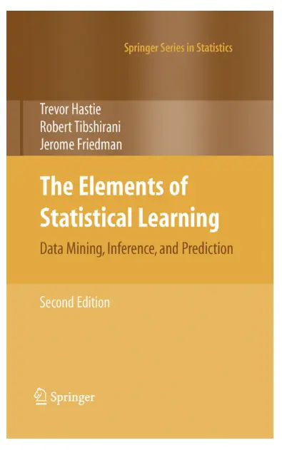
The Elements of Statistical Learning – Trevor Hastie, Robert Tibshirani and Jerome Friedman