Statistical Learning

Let’s start by loading the packages we need in this lab.

## Install packages if necessary 
## (make sure you have the BiocManager package installed)
# pkgs <- c("ISLR2, 
#           "MASS",
#           "glmnet",
#           "monaLisa",
#           "SummarizedExperiment",
#           "ggplot2",
#           "patchwork", 
#           "tidyverse")
# BiocManager::install(pkgs)

## Load packages
suppressPackageStartupMessages({
    library(ISLR2)
    library(MASS)
    library(glmnet)
    library(monaLisa)
    library(SummarizedExperiment)
    library(ggplot2)
    library(patchwork)
    library(tidyverse)
})

1 Overview

1.1 Learning outcomes

understand what a linear model is
understand the different flavors of linear regression and what differentiates them
know what these terms mean: predictor, response, residual, coefficient, least squares
understand bias-variance trade off and collinearity in regression
be able to assess what linear regression fits best to learn what you need from your data

Note that boxes labeled Task will ask you to do follow up analyses or exploration using what has been demonstrated. We will discuss them and go through them together.

1.2 Linear models

Linear models are incredibly useful and powerful in that they allows us to learn something from the data while providing a high degree of interpretability. Given a variable $y$, the model assumes the expected value of $y$ is linear in the inputs $x$. Mathematically, we model $y = \beta_0 + \beta_1x_1 + ... + \beta_px_p + \epsilon$ for $p$ variables or predictors.

1.3 Annotations and vocabulary

There is some vocabulary we will use in this lab, and it’s good to start getting used to these naming conventions if you don’t already know them. We often refer to $y$ as the response or dependent variable, and to $x$ as the predictor or independent variable.

We are learning the linear function $y \sim \hat{f}(x)$. This fit is not perfect, due to measuring errors or if the linear model is a poor representation of $y$. We look at the difference between the observed $y$ and predicted $\hat{y}=\beta_0 + \beta_1x_1 + ... + \beta_px_p$. This difference is called the residual. For each observation $i$, the residual $e_i = y_i - \hat{y_i}$. The least squares method will find beta estimates that minimize the squared sum of these residuals. In other words we want to minimize the the residual sum of squares (RSS) where $RSS=\sum_{i=1}^Ne_i^2$.

1.4 The data sets

1.4.1 Advertising data set

The advertising data set is a simulated data set coming from the “Introduction to Statistical Learning” book by Gareth James, Daniela Witten, Trevor Hastie and Robert Tibshirani.

## Set to the desired working directory (you may change this to suit your wdir)
wdir <- "~/GitHub/raukr-2026/labs/stats"
setwd(wdir)

## Download the dataset
download.file(url = "https://www.statlearning.com/s/Advertising.csv", 
              destfile = file.path(wdir, "assets", "Advertising.csv"))

## Read in the data 
advertisingData <- read.csv(file = "assets/Advertising.csv", 
                            header = TRUE, 
                            row.names = 1)
str(advertisingData)
head(advertisingData)
summary(advertisingData)

'data.frame':   200 obs. of  4 variables:
 $ TV       : num  230.1 44.5 17.2 151.5 180.8 ...
 $ radio    : num  37.8 39.3 45.9 41.3 10.8 48.9 32.8 19.6 2.1 2.6 ...
 $ newspaper: num  69.2 45.1 69.3 58.5 58.4 75 23.5 11.6 1 21.2 ...
 $ sales    : num  22.1 10.4 9.3 18.5 12.9 7.2 11.8 13.2 4.8 10.6 ...

TV	radio	newspaper	sales
230.1	37.8	69.2	22.1
44.5	39.3	45.1	10.4
17.2	45.9	69.3	9.3
151.5	41.3	58.5	18.5
180.8	10.8	58.4	12.9
8.7	48.9	75.0	7.2

       TV             radio          newspaper          sales      
 Min.   :  0.70   Min.   : 0.000   Min.   :  0.30   Min.   : 1.60  
 1st Qu.: 74.38   1st Qu.: 9.975   1st Qu.: 12.75   1st Qu.:10.38  
 Median :149.75   Median :22.900   Median : 25.75   Median :12.90  
 Mean   :147.04   Mean   :23.264   Mean   : 30.55   Mean   :14.02  
 3rd Qu.:218.82   3rd Qu.:36.525   3rd Qu.: 45.10   3rd Qu.:17.40  
 Max.   :296.40   Max.   :49.600   Max.   :114.00   Max.   :27.00

colnames(advertisingData)

[1] "TV"        "radio"     "newspaper" "sales"

sales: sales (in thousands) of the product
TV: advertising budget on TV
radio: advertising budget on the radio
newspaper: advertising budget in newspapers

1.4.2 Credit data set

The Credit data set is a data set coming from the “Introduction to Statistical Learning” book by Gareth James, Daniela Witten, Trevor Hastie and Robert Tibshirani. It contains information on credit card debt for customers, and is available through the R package accompanying the book, called ISLR2.

attach(Credit)
head(Credit)

Income	Limit	Rating	Cards	Age	Education	Own	Student	Married	Region	Balance
14.891	3606	283	2	34	11	No	No	Yes	South	333
106.025	6645	483	3	82	15	Yes	Yes	Yes	West	903
104.593	7075	514	4	71	11	No	No	No	West	580
148.924	9504	681	3	36	11	Yes	No	No	West	964
55.882	4897	357	2	68	16	No	No	Yes	South	331
80.180	8047	569	4	77	10	No	No	No	South	1151

colnames(Credit)

 [1] "Income"    "Limit"     "Rating"    "Cards"     "Age"       "Education"
 [7] "Own"       "Student"   "Married"   "Region"    "Balance"

Income: income in thousands of dollars
Limit: credit limit
Rating: credit rating
Cards: number of credit cards
Age: age of individual
Education: years of education
Own: house ownership
Student: student status
Married: marital status
Region: East, West or South
Balance: average credit card depth of an individual

1.4.3 Prostate data set

The prostate cancer data set comes from The Elements of Statistical Learning book by Trevor Hastie, Robert Tibshirani and Jerome Friedman. The data contains measurements of prostate specific antigen (PSA) and a number of clinical measurements in men who were about to receive a radical prostatectomy.

## Download the dataset
download.file(url = "https://hastie.su.domains/ElemStatLearn/datasets/prostate.data", 
              destfile = file.path(wdir, "assets", "ProstateData.txt"))

## Read in the data 
prostateData <- read.table(file = "assets/ProstateData.txt", 
                           header = TRUE, 
                           sep = "\t", 
                           row.names = 1)
str(prostateData)
head(prostateData)
summary(prostateData)

'data.frame':   97 obs. of  10 variables:
 $ lcavol : num  -0.58 -0.994 -0.511 -1.204 0.751 ...
 $ lweight: num  2.77 3.32 2.69 3.28 3.43 ...
 $ age    : int  50 58 74 58 62 50 64 58 47 63 ...
 $ lbph   : num  -1.39 -1.39 -1.39 -1.39 -1.39 ...
 $ svi    : int  0 0 0 0 0 0 0 0 0 0 ...
 $ lcp    : num  -1.39 -1.39 -1.39 -1.39 -1.39 ...
 $ gleason: int  6 6 7 6 6 6 6 6 6 6 ...
 $ pgg45  : int  0 0 20 0 0 0 0 0 0 0 ...
 $ lpsa   : num  -0.431 -0.163 -0.163 -0.163 0.372 ...
 $ train  : logi  TRUE TRUE TRUE TRUE TRUE TRUE ...

lcavol	lweight	age	lbph	lcp	gleason	pgg45	lpsa	train
-0.5798185	2.769459	50	-1.386294	-1.386294	6	0	-0.4307829	TRUE
-0.9942523	3.319626	58	-1.386294	-1.386294	6	0	-0.1625189	TRUE
-0.5108256	2.691243	74	-1.386294	-1.386294	7	20	-0.1625189	TRUE
-1.2039728	3.282789	58	-1.386294	-1.386294	6	0	-0.1625189	TRUE
0.7514161	3.432373	62	-1.386294	-1.386294	6	0	0.3715636	TRUE
-1.0498221	3.228826	50	-1.386294	-1.386294	6	0	0.7654678	TRUE

     lcavol           lweight           age             lbph        
 Min.   :-1.3471   Min.   :2.375   Min.   :41.00   Min.   :-1.3863  
 1st Qu.: 0.5128   1st Qu.:3.376   1st Qu.:60.00   1st Qu.:-1.3863  
 Median : 1.4469   Median :3.623   Median :65.00   Median : 0.3001  
 Mean   : 1.3500   Mean   :3.629   Mean   :63.87   Mean   : 0.1004  
 3rd Qu.: 2.1270   3rd Qu.:3.876   3rd Qu.:68.00   3rd Qu.: 1.5581  
 Max.   : 3.8210   Max.   :4.780   Max.   :79.00   Max.   : 2.3263  
      svi              lcp             gleason          pgg45       
 Min.   :0.0000   Min.   :-1.3863   Min.   :6.000   Min.   :  0.00  
 1st Qu.:0.0000   1st Qu.:-1.3863   1st Qu.:6.000   1st Qu.:  0.00  
 Median :0.0000   Median :-0.7985   Median :7.000   Median : 15.00  
 Mean   :0.2165   Mean   :-0.1794   Mean   :6.753   Mean   : 24.38  
 3rd Qu.:0.0000   3rd Qu.: 1.1787   3rd Qu.:7.000   3rd Qu.: 40.00  
 Max.   :1.0000   Max.   : 2.9042   Max.   :9.000   Max.   :100.00  
      lpsa           train        
 Min.   :-0.4308   Mode :logical  
 1st Qu.: 1.7317   FALSE:30       
 Median : 2.5915   TRUE :67       
 Mean   : 2.4784                  
 3rd Qu.: 3.0564                  
 Max.   : 5.5829

colnames(prostateData)

 [1] "lcavol"  "lweight" "age"     "lbph"    "svi"     "lcp"     "gleason"
 [8] "pgg45"   "lpsa"    "train"

lcavol: log cancer volume
lweight: log prostate weight
age: individual’s age
lbph: log of benign prostatic hyperplasia amount
svi: seminal vesicle invasion
lcp: log of capsular penetration
gleason: Gleason score
pgg45: percent of Gleason scores 4 or 5 pgg45
lpsa: log of PSA
train: if this will be used as training data. We will ignore this and use all the data since we are interested in learning the relationship between predictors and not using the data to train a model to use for future predictions.

2 Simple linear regression

As the name implies, a simple linear regression predicts a quantitative response $y$ on the basis of a single predictor $x$ and assumes an approximately linear relationship between $x$ and $y$. Mathematically, we can write this linear relationship as \[y = \beta_0 + \beta_1x + \epsilon\] where $\beta_0$ and $\beta_1$ are the intercept term and the coefficient for $x$ respectively. The error term $\epsilon$ captures the noise or lack of fit to the linear equation.

We are going to assume that we are statistical consultants that were hired by a client to investigate the association between advertising and the sales, in thousands of units, of the product in the advertising data set. In other words, we are estimating the beta coefficients in the following equation: $sales = \beta_0 + \beta_1TV + \epsilon$.

The data contains advertising budgets for the product for three different media: TV, radio and newspaper. Can we learn something about the relationship between sales and advertising that can guide or inform future marketing plans?

Let us have a first look at the sales vs TV relationship in the data. Visually, we can see some kind of linear relationship and that sales increases with increasing TV advertising budget. Is there anything else you notice about the spread of the data?

ggplot(advertisingData, aes(x = TV, y = sales)) + 
    geom_point() + 
    theme_bw()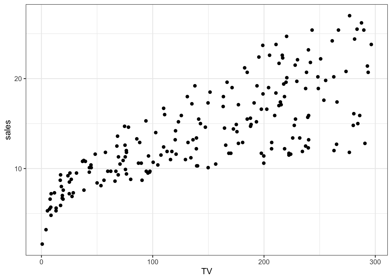

Let’s estimate the beta coefficients and learn the exact linear function capturing this relationship.

## Fit linear model
simpleLinearFit <- lm(sales ~ TV, data = advertisingData) 
simpleLinearFit
names(simpleLinearFit)


Call:
lm(formula = sales ~ TV, data = advertisingData)

Coefficients:
(Intercept)           TV  
    7.03259      0.04754  

 [1] "coefficients"  "residuals"     "effects"       "rank"         
 [5] "fitted.values" "assign"        "qr"            "df.residual"  
 [9] "xlevels"       "call"          "terms"         "model"

Task

Explore the simpleLinearFit object and what it contains. You can make use of the following methods: str(), class(), names() and the $ sign to access slots. You can also refer to the help page of the lm() function to see what it returns. Do you get the same values if you compare the residuals from the simpleLinearFit object to the difference between the sales values and the fitted.values in the simpleLinearFit object?

Let’s plot the linear fit on our original scatter plot.

## prepare to plot
df <- do.call(cbind, list(advertisingData, 
                          residual = simpleLinearFit$residuals, 
                          predictedSales = simpleLinearFit$fitted.values))
beta0 <- simpleLinearFit$coefficients["(Intercept)"]
beta1 <- simpleLinearFit$coefficients["TV"]

## plot
p1 <- ggplot(df, aes(x = TV, y = sales)) + 
    geom_point() +
    geom_abline(intercept = beta0, slope = beta1, color = "firebrick") + 
    theme_bw()

p2 <- p1 + 
    geom_segment(aes(x = TV, xend = TV, y = sales, yend = predictedSales),
                 color = "steelblue")

p1 + p2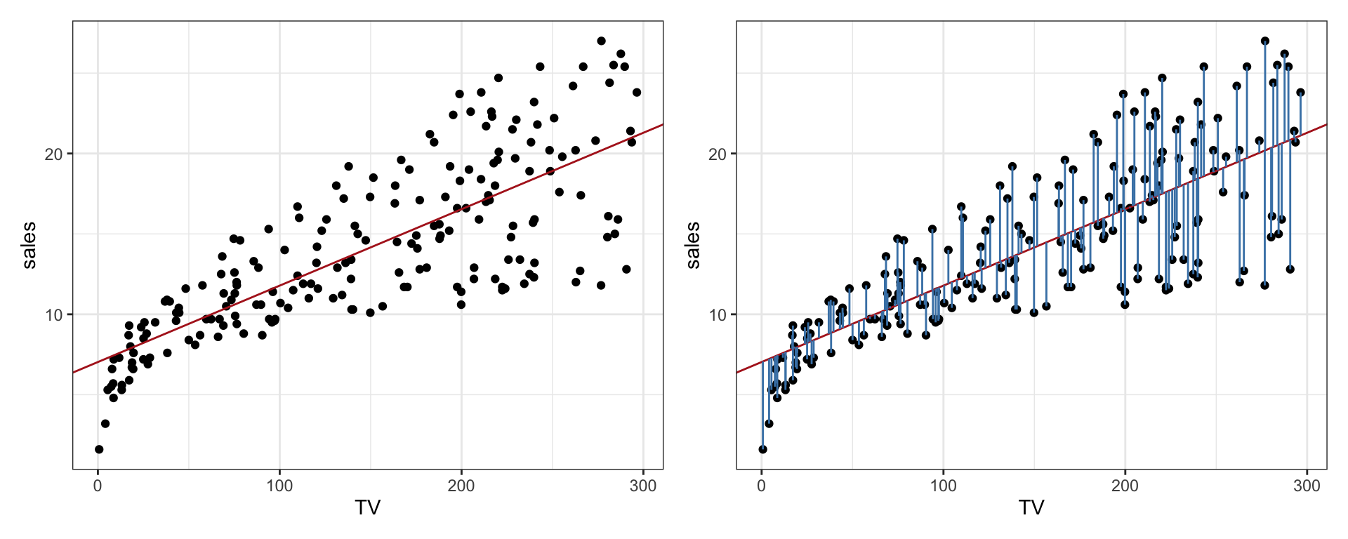

The red line is the linear fit and we can visualize the residuals in blue, which show the difference between predicted and observed sales values. Recall that for each observation $i$, the residual $e_i=y_i-\hat{y_i}$.

Task

Plot the distribution of the residuals. Is it approximately normal?

Now that we have our fit, how do we interpret the values of the beta coefficients and what can we communicate back to our clients? $\beta_0$ is the intercept term, and shows the expected value of $y$ when $x=0$. The slope, $\beta_1$, shows the average increase in $y$ associated with a one-unit increase in $x$. In our example, $\beta_0$ has a value of 7.0326 and $\beta_1$ a value of 0.0475. That means that an additional $1000 spent on TV advertising is associated with selling approximately 47.5 extra units of the product.

Task

Pick either one of the other two advertising budgets, newspaper or radio, and repeat this exercise. What are you expecting based on the scatter plots before doing any fit? Is there a positive relationship to sales, and to what extent? Fit a line and interpret the coefficients. Can you say something about how well the fit captures the trend in the data?

2.1 Assessing the quality of the fit

We will explore two measurements that allow us to assess the quality of the linear regression fit: the residual standard error (RSE) and the $R^2$ statistic.

Recall that we can’t perfectly predict $y$ from $x$ and that there is an associated residual $e$ for each observation showing how much we have deviated from the line. The RSE roughly represents the average amount of deviation from this line, as reflected in its formula: $RSE=\sqrt{\frac{1}{N-2}RSS}$ where N is the number of observations. Let’s have a look at the RSE value in our example. Note that here we have $N-2$ since we have 2 coefficients.

summary(simpleLinearFit)


Call:
lm(formula = sales ~ TV, data = advertisingData)

Residuals:
    Min      1Q  Median      3Q     Max 
-8.3860 -1.9545 -0.1913  2.0671  7.2124 

Coefficients:
            Estimate Std. Error t value Pr(>|t|)    
(Intercept) 7.032594   0.457843   15.36   <2e-16 ***
TV          0.047537   0.002691   17.67   <2e-16 ***
---
Signif. codes:  0 '***' 0.001 '**' 0.01 '*' 0.05 '.' 0.1 ' ' 1

Residual standard error: 3.259 on 198 degrees of freedom
Multiple R-squared:  0.6119,    Adjusted R-squared:  0.6099 
F-statistic: 312.1 on 1 and 198 DF,  p-value: < 2.2e-16

The RSE has a value of 3.26. The observed sales deviate from the true regression line by about 3,260 units on average (since the sales is in thousands of units). Is this something we can live with? What is the mean value of sales in our data set?

## mean sales (in thousdands of units)
mean(advertisingData$sales)

## percentage error
summary(simpleLinearFit)$sigma / mean(advertisingData$sales) * 100

[1] 14.0225
[1] 23.23877

The size of the RSE value will reflect how poorly the model fits the data. However, the RSE is measured in units of $y$ and it is not always clear what a good value should be. The $R^2$ statistic on the other hand represents the proportion of variance explained, meaning it will always have a value between 0 and 1: $R^2=\frac{TSS-RSS}{TSS}$ where $TSS=\sum(y_i-\bar{y})^2$ and $\bar{y}$ is the mean of $y$. TSS is the total sum of squares and measures the total variance in $y$, whereas the RSS can be thought of as measuring the variability that is left unexplained after doing the regression. The $R^2$ value thus reflects the proportion of variability in $y$ that can be explained using $x$ by performing the regression. In our example, $R^2$ has a value of 0.61, meaning that around two thirds of the variability in sales is explained by a linear regression on TV advertising budget. Even though the $R^2$ is nicely interpretable, it can still be difficult to judge what a good value should look like in practice, particularly in fields where data is generated with a degree of experimental noise such as in biology.

Note

Note that in the case of the simple linear regression, the $R^2$ is identical to $Cor(y, \hat{y})^2$.

3 Multiple linear regression

Now that we have a good understanding of the simple linear regression with one dependent variable $x$, let’s extend this problem by including more predictors (dependent variables). Continuing with the advertising data set, can we say something about which kind of advertising has a bigger impact on sales based on the size of the beta coefficients? With more than one predictor, this form of linear regression is called multiple linear regression and is formulated as follows for $p$ predictors: $y = \beta_0 + \beta_1x_1 + \beta_2x_2 + ... + \beta_px_p + \epsilon$.

In the original advertising data, $sales = \beta_0 + \beta_1TV + \beta_2radio + \beta_3newspaper + \epsilon$. As with the simple linear regression, we estimate the beta coefficients to minimize the sum of the squared residuals or the RSS.

We don’t have too many predictors to crowd a pairs plot. Let’s look at all combinations of scatter plots and get a feeling for the data. What can we see?

## visualize the data
pairs(advertisingData, pch = 16)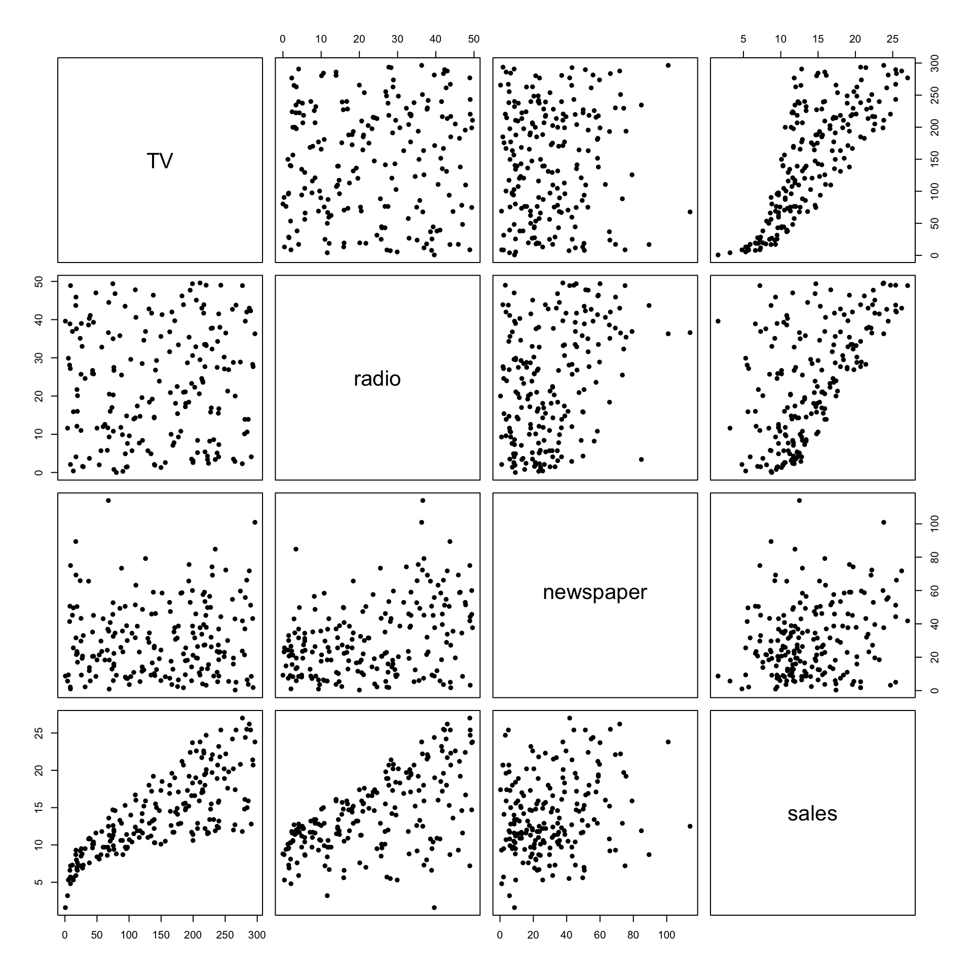

## fit
multipleLinearFit <- lm(sales ~ TV + radio + newspaper, 
                        data = advertisingData) 
multipleLinearFit

## compare to the sales ~ TV fit
summary(simpleLinearFit)


Call:
lm(formula = sales ~ TV + radio + newspaper, data = advertisingData)

Coefficients:
(Intercept)           TV        radio    newspaper  
   2.938889     0.045765     0.188530    -0.001037  


Call:
lm(formula = sales ~ TV, data = advertisingData)

Residuals:
    Min      1Q  Median      3Q     Max 
-8.3860 -1.9545 -0.1913  2.0671  7.2124 

Coefficients:
            Estimate Std. Error t value Pr(>|t|)    
(Intercept) 7.032594   0.457843   15.36   <2e-16 ***
TV          0.047537   0.002691   17.67   <2e-16 ***
---
Signif. codes:  0 '***' 0.001 '**' 0.01 '*' 0.05 '.' 0.1 ' ' 1

Residual standard error: 3.259 on 198 degrees of freedom
Multiple R-squared:  0.6119,    Adjusted R-squared:  0.6099 
F-statistic: 312.1 on 1 and 198 DF,  p-value: < 2.2e-16

summary(multipleLinearFit)


Call:
lm(formula = sales ~ TV + radio + newspaper, data = advertisingData)

Residuals:
    Min      1Q  Median      3Q     Max 
-8.8277 -0.8908  0.2418  1.1893  2.8292 

Coefficients:
             Estimate Std. Error t value Pr(>|t|)    
(Intercept)  2.938889   0.311908   9.422   <2e-16 ***
TV           0.045765   0.001395  32.809   <2e-16 ***
radio        0.188530   0.008611  21.893   <2e-16 ***
newspaper   -0.001037   0.005871  -0.177     0.86    
---
Signif. codes:  0 '***' 0.001 '**' 0.01 '*' 0.05 '.' 0.1 ' ' 1

Residual standard error: 1.686 on 196 degrees of freedom
Multiple R-squared:  0.8972,    Adjusted R-squared:  0.8956 
F-statistic: 570.3 on 3 and 196 DF,  p-value: < 2.2e-16

We interpret $\beta_j$ as the average effect on $y$ of a one unit increase in $x_j$, holding all other predictors fixed. Spending an additional $1,000 on radio advertising is associated with an average increase in around 189 units of additional sales. How do the coefficients for all predictors in the multiple linear regression compare to the coefficients if we were to do a simple linear regression separately per predictor? What do you notice about the newspaper predictor and the (adjusted - adjusted for the numebr of predictors) $R^2$ values?

The multiple linear regression allows us to assess the contribution of a predictor in explaining the response vector in context with the other predictors and allows us to assess the relative contributions of each predictor.

4 Interaction terms

In our advertising data, we have seen that both the TV and radio are media whose budgets contribute towards explaining the sales and both have (significantly) positive coefficient estimates. But what can we say about their joint contribution towards the sales at the same time? What if each predictor is associated with sales in a different way, and if we were to take them together the beta coefficient for the TV and radio budget would be even bigger? These are questions we currently have, and which we can address by including an interaction term, reflecting the product of the TV and radio predictors.

We can represent the predictors in a matrix form $X$ called the predictor matrix. The equation $y = \beta_0 + \beta_1x_1 + \beta_2x_2 + ... + \beta_px_p + \epsilon$ can be rewritten as $y = \beta.X + \epsilon$ where $\beta$ is the vector of beta coefficients which we are estimating. $X$ includes the intercept term which is a vector of 1s (multiplying 1 by the estimated intercept yields the intercept). In R we can use the model.matrix() function to create this matrix (the lm() function does this internally).

To add an interaction term, we can simply add TV:radio into the lm() function, or we can use TV*radio which will expand into TV + radio + TV:radio.

## create predictor matrix (you may recognize this as the design matrix)
X <- model.matrix(~ TV + radio + newspaper + TV:radio, 
                  data = advertisingData)
head(X)

## linear regression (all ways below work)
#lm(sales ~ TV + radio + TV:radio + newspaper, data = advertisingData)
#lm(sales ~ TV*radio + newspaper, data = advertisingData)
fit <- lm(advertisingData$sales ~ X + 0)
summary(fit)

  (Intercept)    TV radio newspaper TV:radio
1           1 230.1  37.8      69.2  8697.78
2           1  44.5  39.3      45.1  1748.85
3           1  17.2  45.9      69.3   789.48
4           1 151.5  41.3      58.5  6256.95
5           1 180.8  10.8      58.4  1952.64
6           1   8.7  48.9      75.0   425.43

Call:
lm(formula = advertisingData$sales ~ X + 0)

Residuals:
    Min      1Q  Median      3Q     Max 
-6.2929 -0.3983  0.1811  0.5957  1.5009 

Coefficients:
              Estimate Std. Error t value Pr(>|t|)    
X(Intercept) 6.728e+00  2.533e-01  26.561  < 2e-16 ***
XTV          1.907e-02  1.509e-03  12.633  < 2e-16 ***
Xradio       2.799e-02  9.141e-03   3.062  0.00251 ** 
Xnewspaper   1.444e-03  3.295e-03   0.438  0.66169    
XTV:radio    1.087e-03  5.256e-05  20.686  < 2e-16 ***
---
Signif. codes:  0 '***' 0.001 '**' 0.01 '*' 0.05 '.' 0.1 ' ' 1

Residual standard error: 0.9455 on 195 degrees of freedom
Multiple R-squared:  0.9961,    Adjusted R-squared:  0.996 
F-statistic:  9972 on 5 and 195 DF,  p-value: < 2.2e-16

What do you notice about the beta coefficients and the adjusted R-squared?

5 Categorical variables

So far we have dealt with quantitative values of the predictors. What if we have a qualitative variable for example indicating presence or absence? What happens in the linear fit when such a predictor exists? To illustrate this, we will use another data set, namely the Credit data set, where we have a mixture of quantitative and qualitative variables.

head(Credit)

Income	Limit	Rating	Cards	Age	Education	Own	Student	Married	Region	Balance
14.891	3606	283	2	34	11	No	No	Yes	South	333
106.025	6645	483	3	82	15	Yes	Yes	Yes	West	903
104.593	7075	514	4	71	11	No	No	No	West	580
148.924	9504	681	3	36	11	Yes	No	No	West	964
55.882	4897	357	2	68	16	No	No	Yes	South	331
80.180	8047	569	4	77	10	No	No	No	South	1151

To illustrate, we will use the balance variable as the response vector and investigate differences in credit card balance between those who own a house and those who don’t: $balance = \beta_0 + \beta_1Own + \epsilon$. The categorical variable Own can be represented as a vector of 0s and 1s indicating where an individual owns a house. This is also called a dummy variable and takes two possible values: $x_i=1$ if the $i^{th}$ person owns a house and $x_i=0$ otherwise. This results in $y_i = \beta_0 + \beta_1 +\epsilon_i$ if person $i$ owns a house and in $y_i = \beta_0 +\epsilon_i$ if person $i$ does not own a house. $\beta_0$ is now interpreted as the average credit balance for those who do not own, $\beta_0+\beta_1$ the average credit balance for those who do own, and $\beta_1$ reflects the average difference in credit balance between home owners and non-owners. What is the average credit card debt for home owners in the Credit data set?

## fit
lm(Balance ~ Own, data = Credit)


Call:
lm(formula = Balance ~ Own, data = Credit)

Coefficients:
(Intercept)       OwnYes  
     509.80        19.73

Task

Use the model.matrix() function to see what the predictor matrix looks like. What do you see?

Task

Examine the Credit data set. Which columns represent categorical variables? Pick one categorical variable and do a linear fit. Notice that categorical variables are represented as $l-1$ dummy variables, where $l$ is the number of levels.

Example:

X <- model.matrix(~ Region, 
                  data = Credit)
head(X)

  (Intercept) RegionSouth RegionWest
1           1           1          0
2           1           0          1
3           1           0          1
4           1           0          1
5           1           1          0
6           1           1          0

Can you think of another way to represent categorical variables?

6 Robust regression

So far in the linear fit, the coefficients are estimated using the least squares method by minimizing the sum of squared residuals: $\min\limits_{\beta}\sum_{i=1}^{N}e_{i}^{2}$ where the residual for the $i^{th}$ observation $e_{i} = (y_i - \hat{y_i})$. What if we had outlier points which would result in large residuals? Does this have an impact on the linear fit? To illustrate this, we will add artificial observations to the advertising data set which deviate quite a bit from the rest of the trend in the data and visualize below.

## add outlier points
nOutliers <- 30
advertisingOutlData <- rbind(advertisingData, 
                         data.frame(TV = runif(n = nOutliers, min = 50, max = 150), 
                                    radio = runif(n = nOutliers, min = 10, max = 15), 
                                    newspaper = runif(n = nOutliers, min = 10, max = 30), 
                                    sales = runif(n = nOutliers, min = 20, max = 30)))

## visualize
ggplot(advertisingOutlData, aes(x = TV, y = sales)) + 
    geom_point() + 
    theme_bw()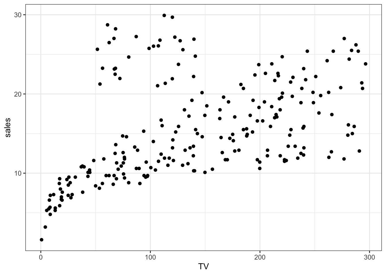

## fit linear model with lm()
lmFit <- lm(sales ~ TV, data = advertisingOutlData) 

## prepare to plot
df <- do.call(cbind, list(advertisingOutlData, 
                          residual = lmFit$residuals, 
                          predictedSales = lmFit$fitted.values))
beta0lm <- lmFit$coefficients["(Intercept)"]
beta1lm <- lmFit$coefficients["TV"]

## plot
ggplot(df, aes(x = TV, y = sales)) + 
    geom_point() +
    geom_abline(intercept = beta0lm, slope = beta1lm, color = "firebrick") + 
    theme_bw() + 
    geom_segment(aes(x = TV, xend = TV, y = sales, yend = predictedSales),
                 color = "steelblue")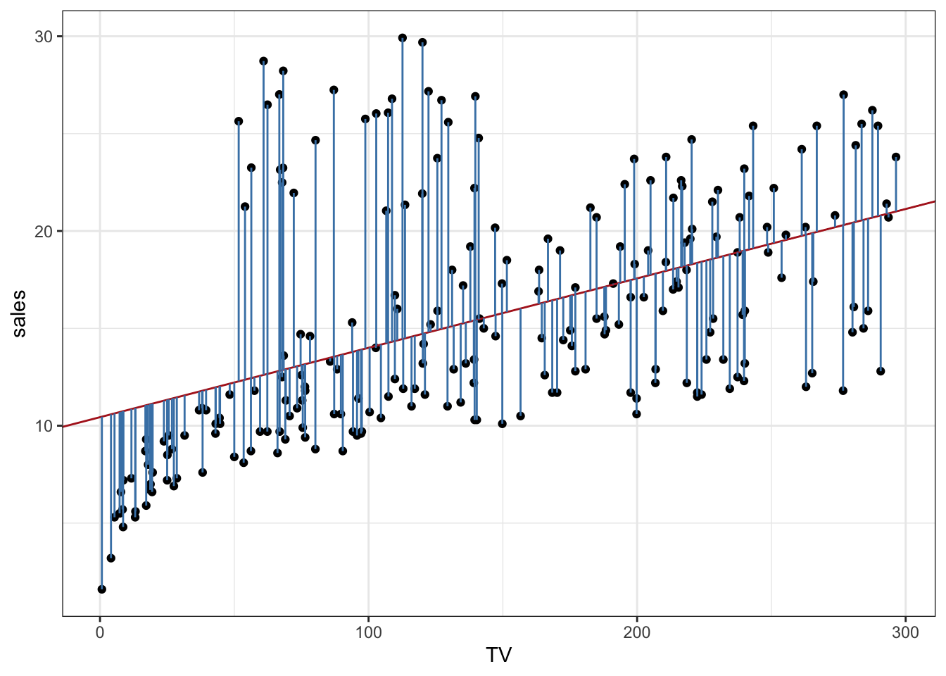

What do you notice about the fitted line and the residuals?

Currently, all residuals contribute equally in the summation we are minimizing. With a robust linear regression, the very big residuals can be weighted less and therefore contribute less to the total sum of the squared residuals.

## robust linear fit
robustFit <- rlm(sales ~ TV, data = advertisingOutlData) 
robustFit

## prepare to plot
df <- do.call(cbind, list(advertisingOutlData, 
                          predictedSales = robustFit$fitted.values, 
                          weightedResidual = robustFit$wresid, 
                          weight = robustFit$w))
beta0rlm <- robustFit$coefficients["(Intercept)"]
beta1rlm <- robustFit$coefficients["TV"]

## plot
ggplot(df, aes(x = TV, y = sales)) + 
    geom_point() +
    geom_abline(aes(intercept = beta0lm, 
                    slope = beta1lm,
                    color = "Linear regression")) + 
    geom_abline(aes(intercept = beta0rlm, 
                    slope = beta1rlm,
                    color = "Robust regression")) +
    geom_abline(aes(intercept = beta0, 
                    slope = beta1,
                    color = "Original linear regression (without outliers)")) +
    scale_color_manual(name = "Model", 
                       values = c("Linear regression" = "firebrick", 
                                  "Robust regression" = "forestgreen", 
                                  "Original linear regression (without outliers)" = "steelblue")) +
    theme_bw()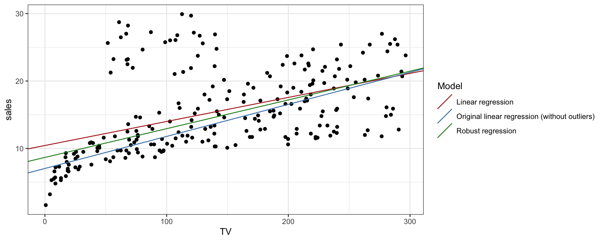

Call:
rlm(formula = sales ~ TV, data = advertisingOutlData)
Converged in 6 iterations

Coefficients:
(Intercept)          TV 
 8.66918431  0.04263939 

Degrees of freedom: 230 total; 228 residual
Scale estimate: 4.21

Note that the fitted line using the robust regression better fits the trend in the non-outlier points and gets closer to the original fit we had on the data before adding the so-called outliers. The robust regression can have useful applications for example in data sets where we are interested in selecting outliers which deviate from an expected trend, and we want to capture a good fit on that trend.

Let’s plot the same scatter plot, coloring by the weight each point receives, reflecting its contribution to the sum of the squared residuals. What do you see? Seeing a scatter plot like this, and assuming we are interested in the outlier points in the cloud above the rest of the data, as they seem to be capturing a signal deviating from an expected background trend, how can we select that group in a data-driven manner?

## plot coloring by weight
p1 <- ggplot(df, aes(x = TV, y = sales)) + 
    geom_point(aes(color = weight)) +
    geom_abline(intercept = beta0rlm, 
                    slope = beta1rlm,
                    color = "forestgreen") +
    theme_bw() 

## naturally define cutoffs for outliers
p2 <- ggplot(df, aes(x = 1 - weight)) + 
    geom_density() + 
    theme_bw() 
df$selected <- 1 - df$weight > 0.3

p3 <- ggplot(df, aes(x = TV, y = sales)) + 
    geom_point(aes(color = selected)) +
    geom_abline(intercept = beta0rlm, 
                slope = beta1rlm,
                color = "forestgreen") +
    theme_bw() 

p1 + p2 + p3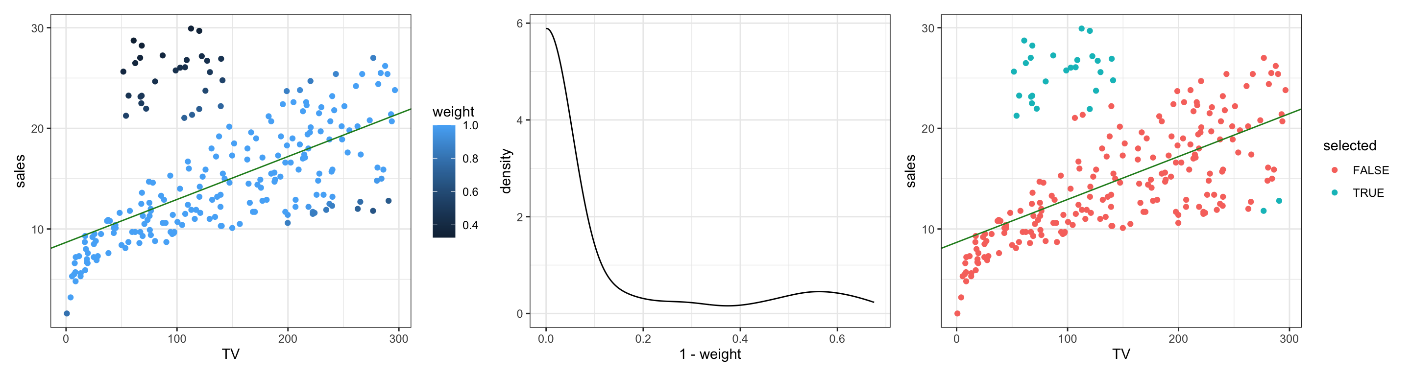

We have done this selection very exploratively, to illustrate that it is possible to select outliers in a data-driven way with robust statistical methods and continue with downstream analyses. Note that in these cases we are actually interested in outliers that deviate from an expected technical or background trend and in properly fitting that expected trend.

Task

Using the credit data set, model the relationship between Income (response) and Age (predictor). We will assume that there is a general trend between both variables and that there are some individuals who deviate from this trend. We wish to reasonably select these individuals and fit the background trend.

7 Note on non-linearities

The flexibility and power of linear models is not to be underestimated. So far we have used the predictors as they are in our examples. However there is nothing preventing us from using non-linear transformations of these predictors, such as the square root ($\sqrt{(x)}$), a log transformation ($log2(x)$) or raising it to the power of some number (such as $x^2$ or $x^3$), to mention a few. The relationship between predictors, whatever transformation they may have taken, is still linear in the context of the linear model. Linear models assume a linear relationship between the predictors and the expected value of the response. Using transformed values of the predictors or response does not violate this, merely how we interpret the fit.

8 Bias-variance trade off

So far with the least squares approach, we have estimated beta coefficients such that the residual sum of squares is minimized. This simple approach while powerful, does not always work best in practice on real world data. If we learn the model on one data set, do we get the same coefficients estimated on another data set? Data can inherently vary due to measuring errors for example, and so we can easily end up over-fitting the coefficients in one data set. Additionally, suppose that two predictors are highly correlated with each other but not with the response. If both predictors get equal coefficient values but opposite signs they cancel each other out. In such cases the coefficients can get arbitrarily large without adding much to the RSS. We again suffer at getting good estimates of the beta coefficients and reliably interpreting them. To overcome these problems and estimate beta coefficients that are more robust and representative, shrinkage methods have been proposed by imposing a penalty on the size of the beta coefficients. This problem is known as the bias-variance trade off, since the beta estimates will vary less with such imposed penalties at the expense of being slightly more biased since we are deliberately constraining them.

Task

Pick one of the two data sets we have explored so far (Advertising or Credit), randomly split the observations into two and then do a linear fit on each subset. Do you get identical beta estimates or do they vary? The code below demonstrates this on the Advertising data set.

## set seed for random sampling (for reproducibility)
set.seed(123)
i <- sample(x = nrow(advertisingData), 
            size = floor(nrow(advertisingData)/2))

## subset data
set1 <- advertisingData[i, ]
set2 <- advertisingData[-i, ]

## fit model
fit1 <- lm(formula = sales ~ TV + radio + newspaper, data = set1)
fit2 <- lm(formula = sales ~ TV + radio + newspaper, data = set2)

## compare fits
fit1
fit2


Call:
lm(formula = sales ~ TV + radio + newspaper, data = set1)

Coefficients:
(Intercept)           TV        radio    newspaper  
    3.68340      0.04354      0.18608     -0.01352  


Call:
lm(formula = sales ~ TV + radio + newspaper, data = set2)

Coefficients:
(Intercept)           TV        radio    newspaper  
   2.367604     0.047332     0.190075     0.008738

We see that the beta estimates vary. For newspaper they can even have opposite signs. This is perhaps to be expected because data varies, and important to keep in mind as we interpret the numerical values of these coefficients.

9 Shrinkage methods

9.1 Ridge regression

The ridge regression penalizes the beta coefficients by putting a limit on the sum of the squared coefficients. This is done by adding a penalty term $\lambda$ as follows when estimating the beta coefficients:

\[ \hat{\beta}=\min\limits_{\beta}\{\sum_{i=1}^N (y_i - \beta_0 - \sum_{j=1}^px_{ij}\beta_j)^2 + \lambda \sum_{j=1}^p\beta_j^2 \} \]

Notice that in addition to the RSS (first part of the equation) we are penalizing the sum of the squared beta coefficients. When is the above equation identical to the RSS? How do you think the size of $\lambda$ impacts the shrinkage?

The ridge regression shrinks the values of the estimated beta coefficients towards zero. However they are not equal to zero and every coefficient will have an estimated value. To apply the shrinkage regressions, we will make use of the functions from the glmnet package and use the Credit data set. Note that here we will represent the predictors in a matrix $X$. We will focus on the quantitative variables in the Credit data set, but these methods can be used on the whole data set.

## prepare to fit
y <- Credit$Balance
X <- model.matrix(Balance ~ 0 + Income + Limit + Rating + Cards + Age + Education, 
                  data = Credit)
head(X)

## fit
## note that internally, glmnet by default standardizes the predictors 
## ... but returns the beta estimates in the original space
ridgeFit <- glmnet(x = X, y = y, alpha = 0)
#plot(ridgeFit)

## examine the beta estimate for each lambda 
head(ridgeFit$lambda)
ridgeFit$beta[1:6, 1:6]
ncol(ridgeFit$beta) == length(ridgeFit$lambda)

## prepare to plot
betaMat <- as.matrix(ridgeFit$beta)
colnames(betaMat) <- ridgeFit$lambda
df <- betaMat |>
    as.data.frame() |>
    rownames_to_column("predictor") |>
    pivot_longer(
        -predictor,
        names_to = "lambda",
        values_to = "coefficient",
        names_transform = list(lambda = as.numeric)
    )

## plot
p1 <- ggplot(df,
       aes(lambda, coefficient, colour = predictor)) +
  geom_line() +
  theme_bw()
p2 <- p1 +
    coord_cartesian(xlim = c(0, 1e4))
p1 / p2 + plot_layout(guides = 'collect')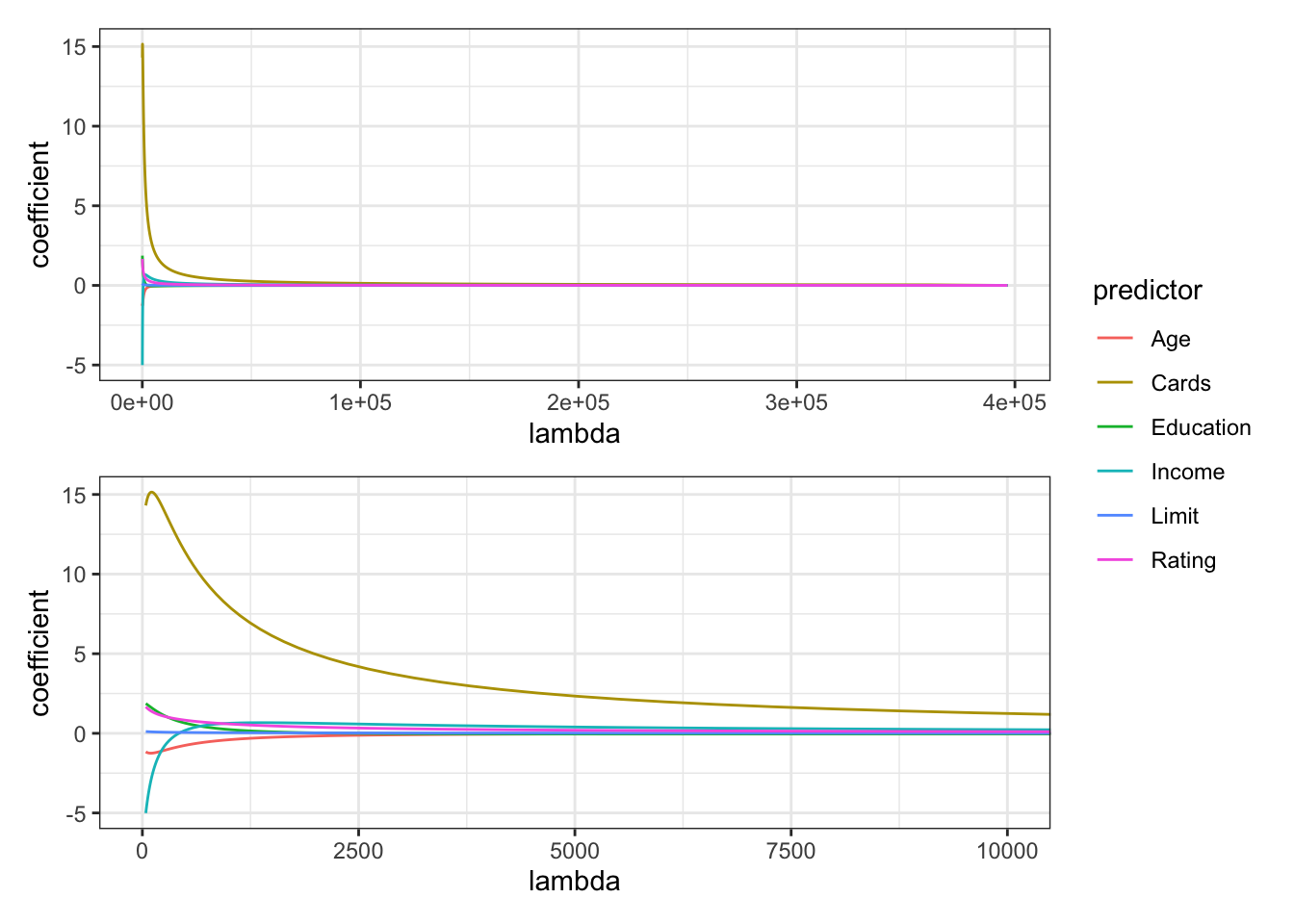

   Income Limit Rating Cards Age Education
1  14.891  3606    283     2  34        11
2 106.025  6645    483     3  82        15
3 104.593  7075    514     4  71        11
4 148.924  9504    681     3  36        11
5  55.882  4897    357     2  68        16
6  80.180  8047    569     4  77        10
[1] 396562.7 361333.2 329233.3 299985.1 273335.3 249052.9
6 x 6 sparse Matrix of class "dgCMatrix"
                     s0            s1            s2            s3            s4
Income     6.109458e-36  7.647903e-03  8.389471e-03  0.0092025091  1.009382e-02
Limit      1.733710e-37  2.174471e-04  2.385764e-04  0.0002617513  2.871682e-04
Rating     2.592162e-36  3.251173e-03  3.567090e-03  0.0039135918  4.293615e-03
Cards      2.927975e-35  3.676476e-02  4.034159e-02  0.0442655953  4.857030e-02
Age        4.940545e-38  5.089846e-05  5.466277e-05  0.0000585505  6.252434e-05
Education -1.197943e-36 -1.490183e-03 -1.633669e-03 -0.0017907777 -1.962763e-03
                     s5
Income     1.107082e-02
Limit      3.150422e-04
Rating     4.710376e-03
Cards      5.329244e-02
Age        6.653337e-05
Education -2.150985e-03
[1] TRUE

Notice that we get different beta estimates with different penalty values. As the penalty increases, the coefficient values decrease or shrink due to heavier penalization. Choosing the right penalty is therefore critical and can have a big impact on our estimates. How can we choose a reasonable $\lambda$ value? A common method is to do cross-validation. For a chosen set of lambdas, the cross-validation error for each value of lambda is calculated, and finally the lambda value which gives the smallest error (lambda.min) is chosen and the model is re-fit with that penalty value. Another common choice is lambda.1se which is where the cross-validated error is within one standard error of the minimum.

## fit with cross validation
ridgeFit <- cv.glmnet(x = X, y = y, alpha = 0)

## plot
plot(ridgeFit)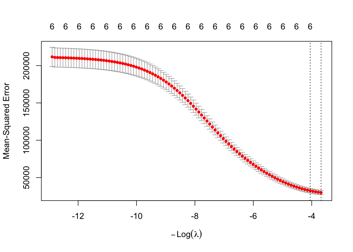

## explore
ridgeFit$lambda.min
ridgeFit$lambda.1se
coef(ridgeFit, s = "lambda.1se")

[1] 39.65627
[1] 57.53446
7 x 1 sparse Matrix of class "dgCMatrix"
              lambda.1se
(Intercept) -346.4443116
Income        -4.2386941
Limit          0.1056099
Rating         1.5709743
Cards         14.7558569
Age           -1.2117421
Education      1.8003424

Task

Do a multiple linear regression on the same data we used in the ridge regression and compare the estimates for the beta coefficients.

9.2 Lasso regression

The Lasso regression also imposes a penalty on the size of the coefficients. However it does so slightly differently, namely by penalizing and thus limiting the sum of the absolute beta values. This has the wonderful effect of resulting in a selection of predictors by setting the coefficients of the uninteresting ones which don’t contribute much to the response to zero. Predictors with non-zero coefficients are considered selected. The beta coefficients are estimated, minimizing the following:

\[ \hat{\beta}=\min\limits_{\beta}\{\frac{1}{2}\sum_{i=1}^N (y_i - \beta_0 - \sum_{j=1}^px_{ij}\beta_j)^2 + \lambda \sum_{j=1}^p|\beta_j| \} \]

## fit
lassoFit <- glmnet(x = X, y = y, alpha = 1)
#plot(lassoFit)

## examine the beta estimate for each lambda 
ncol(lassoFit$beta) == length(lassoFit$lambda)

## prepare to plot
betaMat <- as.matrix(lassoFit$beta)
colnames(betaMat) <- lassoFit$lambda
df <- betaMat |>
    as.data.frame() |>
    rownames_to_column("predictor") |>
    pivot_longer(
        -predictor,
        names_to = "lambda",
        values_to = "coefficient",
        names_transform = list(lambda = as.numeric)
    )

## plot
p1 <- ggplot(df,
       aes(lambda, coefficient, colour = predictor)) +
  geom_line() +
  theme_bw()
p2 <- p1 +
    coord_cartesian(xlim = c(0, 200))
p1 / p2 + plot_layout(guides = 'collect')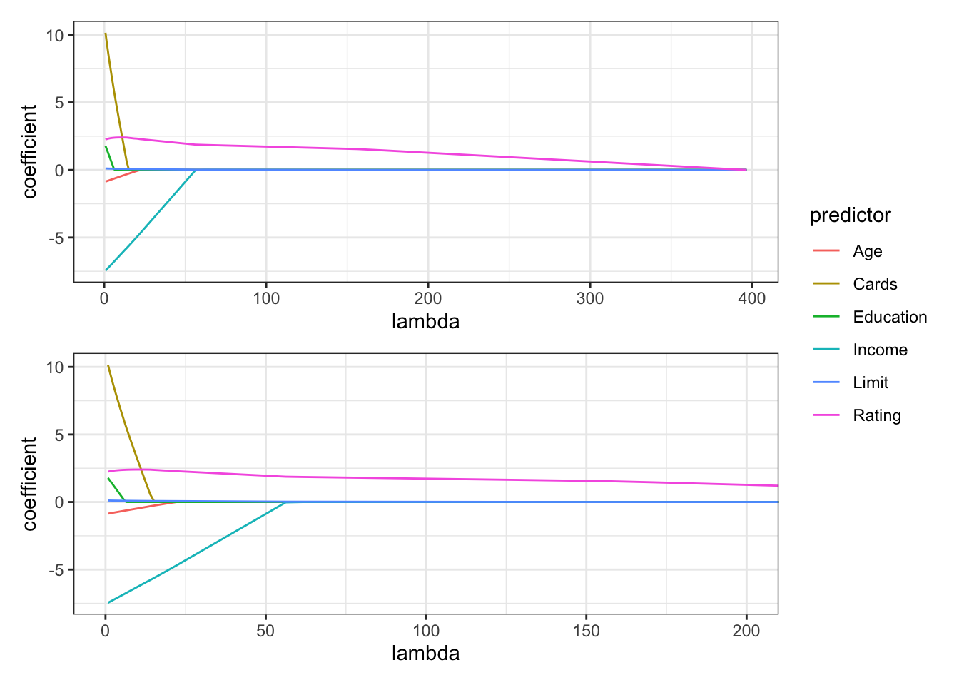

[1] TRUE

How do these plots compare to that of the ridge regression? What do you think it means when a predictor gets set to zero before another one (e.g. Cards and Income)?

## fit with cross validation
lassoFit <- cv.glmnet(x = X, y = y, alpha = 1)

## plot
plot(lassoFit)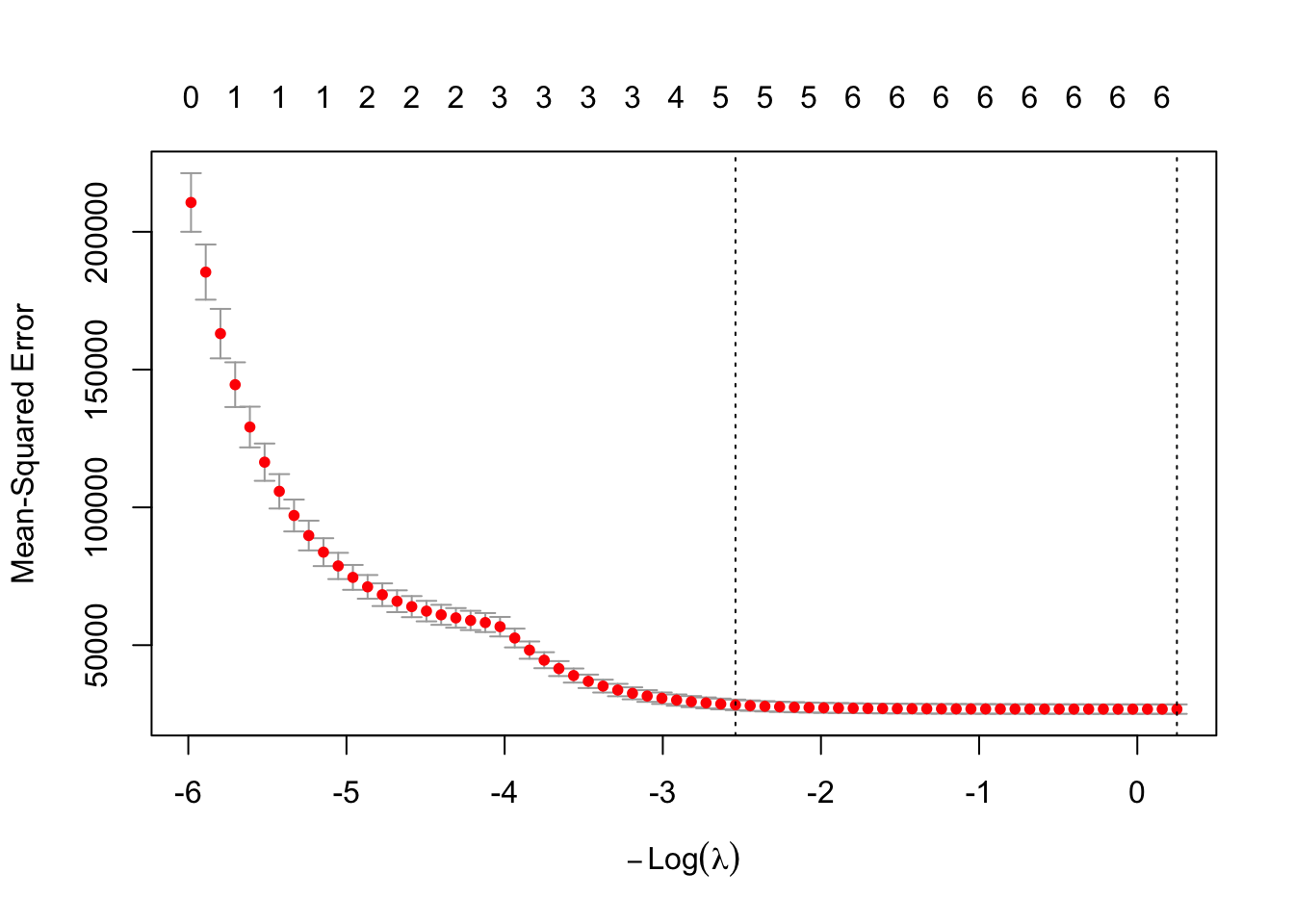

## explore
lassoFit
lassoFit$lambda.min
lassoFit$lambda.1se
coef(lassoFit, s = "lambda.1se")


Call:  cv.glmnet(x = X, y = y, alpha = 1) 

Measure: Mean-Squared Error 

    Lambda Index Measure   SE Nonzero
min  0.778    68   26782 1720       6
1se 12.687    38   28328 1928       5
[1] 0.7784687
[1] 12.6871
7 x 1 sparse Matrix of class "dgCMatrix"
               lambda.1se
(Intercept) -415.71434470
Income        -5.92821076
Limit          0.07769086
Rating         2.40096183
Cards          1.37595158
Age           -0.36615904
Education      .

Is there a coefficient which got set to zero and where does it lie on the plot showing coefficient estimates as a function of the penalty?

9.2.1 Note on collinearity

Since the lasso regression selects the variables that best explain the response vector, there is no need to choose variables which don’t contribute nor to select variables which don’t add much additional value. Consider two predictors which both contribute to the response vector, and which are highly correlated to each other. It is enough to select one of them to be able to explain the response and the model rather thinks there is no need to be redundant and select the second predictor if it doesn’t add or explain much more. This is something one should certainly be aware of and consider in regression.

Let’s go back to our example and look at the correlation structure of our predictor matrix, as well as the correlation to the response vector.

cor(X)

               Income       Limit      Rating       Cards         Age
Income     1.00000000  0.79208834  0.79137763 -0.01827261 0.175338403
Limit      0.79208834  1.00000000  0.99687974  0.01023133 0.100887922
Rating     0.79137763  0.99687974  1.00000000  0.05323903 0.103164996
Cards     -0.01827261  0.01023133  0.05323903  1.00000000 0.042948288
Age        0.17533840  0.10088792  0.10316500  0.04294829 1.000000000
Education -0.02769198 -0.02354853 -0.03013563 -0.05108422 0.003619285
             Education
Income    -0.027691982
Limit     -0.023548534
Rating    -0.030135627
Cards     -0.051084217
Age        0.003619285
Education  1.000000000

cor(X, y)

                  [,1]
Income     0.463656457
Limit      0.861697267
Rating     0.863625161
Cards      0.086456347
Age        0.001835119
Education -0.008061576

From the lasso fit, Rating was selected and had a beta coefficient of 2.401. Compare to that of the Limit predictor. What do you notice about the correlation between Ratings and Limit to each other and to the response?

9.3 Elastic net regression

We won’t dive too deep here, but it is worth mentioning the elastic net. The elastic net is an interesting situation or compromise between the ridge and lasso regressions. You may have noticed that we needed to specify an alpha parameter in the glmnet function to perform the ridge and lasso regressions with alphas of 0 and 1 respectively. The elastic net selects variables like the lasso and shrinks the coefficients of correlated predictors like the ridge using the following penalty:

\[ \lambda \sum_{j=1}^p(\alpha|\beta_j| + (1-\alpha)\beta_j^2) \]

Alpha is a value between 0 and 1 and will dictate how close the regression is to a lasso ($\alpha=1$) or a ridge ($\alpha=0$). The choice in alpha value can be quite tricky. In practice we try a few values, keeping in mind what we know about the correlation structure in our data set, and see what makes sense.

9.3.1 Fit with `alpha=0.5`

## fit with alpha = 0.5
elasticNetFit <- glmnet(x = X, y = y, alpha = 0.5)

## examine the beta estimate for each lambda 
ncol(elasticNetFit$beta) == length(elasticNetFit$lambda)

## prepare to plot
betaMat <- as.matrix(elasticNetFit$beta)
colnames(betaMat) <- elasticNetFit$lambda
df <- betaMat |>
    as.data.frame() |>
    rownames_to_column("predictor") |>
    pivot_longer(
        -predictor,
        names_to = "lambda",
        values_to = "coefficient",
        names_transform = list(lambda = as.numeric)
    )

## plot
p1 <- ggplot(df,
       aes(lambda, coefficient, colour = predictor)) +
  geom_line() +
  theme_bw()
p2 <- p1 +
    coord_cartesian(xlim = c(0, 200))
p1 / p2 + plot_layout(guides = 'collect')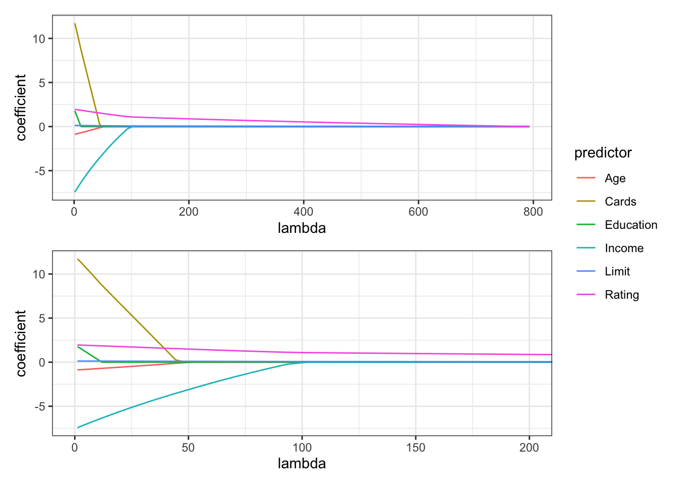

[1] TRUE

10 Stability selection

Although these methods could also fall under shrinkage methods since they do make use of them, they offer additional gains where typical regression methods fail, such as when the number of predictors exceeds the number of observations. The idea behind stability selection is to apply the regression of choice on several subsets of the data, and select the predictors which consistently pop up. Lasso stability selection will apply the lasso regression on subsets of the data and return a selection probability for each predictor which is the number of times it was selected divided by the total number of times a regression was performed. The authors of these methods introduced a new form of regularization with the randomized lasso stability selection. There, a weakness parameter is additionally used to vary the lasso penalty term $\lambda$ to a randomly chosen value between $[\lambda, \lambda/weakness]$ for each predictor. This type of regularization has advantages in cases where the number of predictors exceeds the number of observations, in selecting variables consistently, demonstrating better error control and not depending strongly on the penalization parameter (Meinshausen and Bühlmann 2010).

We will apply the randomized lasso stability selection using the monaLisa package. Have a look at the help page of the randLassoStabSel() function for more details.

## stability selection
randLasso <- randLassoStabSel(x = X, 
                              y = y, 
                              weakness = 0.8, 
                              cutoff = 0.6, 
                              PFER = 1)

## selected predictors
randLasso$selected
randLasso$selProb
randLasso$selAUC  # Area under the curve of the stability paths

## plot stability paths
plotStabilityPaths(randLasso)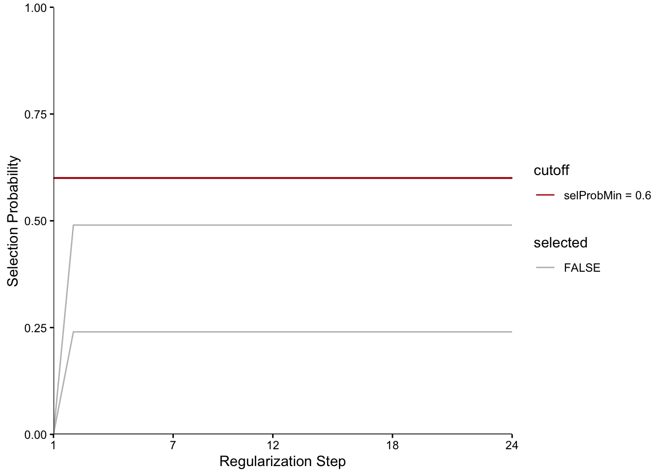

[1] FALSE FALSE FALSE FALSE FALSE FALSE
[1] 0.00 0.49 0.24 0.00 0.00 0.00
   Income     Limit    Rating     Cards       Age Education 
0.0000000 0.4695833 0.2300000 0.0000000 0.0000000 0.0000000

This plot shows the selection probability or each predictor (line) as a function of the regularization step, with weaker regularization going from left to right. These so called stability paths can be quite informative, as an indicator of which predictor(s) gets selected first, if it stays up and how well the selected supposedly meaningful predictors separate from the noisy rest.

In our example nothing gets selected. In practice, randomized stability selection is quite conservative, preferring to select nothing rather than something false. Our choice in parameter values depends on how stringent we want to be and how strong the signal in the data is. For more stringent selections, one may decrease the value of the weakness parameter which will make it harder for a variable to get selected. The user is in control of false discoveries with the PFER parameter, which indicates the number of falsely selected variables. As for the selection probability cutoff, Meinshausen and Bühlmann (2010) argue that values in the range of [0.6, 0.9] should give similar results.

Task

Apply the stability selection method of choice (lasso or randomized) on the prostate cancer data set. Decide on the parameter values and play with them. Examine the output of randLassoStabSel() and plot the stability paths. What are you selecting? Explore the available plotting functions plotStabilityPaths() and plotSelectionProb().

11 Bonus exercise

11.1 Option A

Use the prostate cancer data set and apply a ridge regression, lasso regression and lasso stability selection. Compare the coefficients you are getting and what gets selected, keeping in mind what the correlation structure looks like as well in the predictor matrix.

11.2 Option B

Think about if/how you can use these methods in your projects and which flavor of them would best suit your needs.

12 Resources

A lot of the ideas and material presented in this lab were constructed using the following books:

An Introduction to Statistical Learning with applications in R by Gareth James, Daniela Witten, Trevor Hastie and Robert Tibshirani.
The Elements of Statistical Learning by Trevor Hastie, Robert Tibshirani and Jerome Friedman.

13 Session

Click here

date()
sessionInfo()

[1] "Tue Aug 18 09:01:10 2026"
R version 4.6.0 (2026-04-24)
Platform: aarch64-apple-darwin23
Running under: macOS Sequoia 15.7.7

Matrix products: default
BLAS:   /Library/Frameworks/R.framework/Versions/4.6/Resources/lib/libRblas.0.dylib 
LAPACK: /Library/Frameworks/R.framework/Versions/4.6/Resources/lib/libRlapack.dylib;  LAPACK version 3.12.1

locale:
[1] C/UTF-8/C/C/C/C

time zone: Europe/Stockholm
tzcode source: internal

attached base packages:
[1] stats4    stats     graphics  grDevices utils     datasets  methods  
[8] base     

other attached packages:
 [1] lubridate_1.9.5             forcats_1.0.1              
 [3] stringr_1.6.0               dplyr_1.2.1                
 [5] purrr_1.2.2                 readr_2.2.0                
 [7] tidyr_1.3.2                 tibble_3.3.1               
 [9] tidyverse_2.0.0             patchwork_1.3.2            
[11] ggplot2_4.0.3               SummarizedExperiment_1.42.0
[13] Biobase_2.72.0              GenomicRanges_1.64.0       
[15] Seqinfo_1.2.0               IRanges_2.46.0             
[17] S4Vectors_0.50.1            BiocGenerics_0.58.1        
[19] generics_0.1.4              MatrixGenerics_1.24.0      
[21] matrixStats_1.5.0           monaLisa_1.18.0            
[23] glmnet_5.0                  Matrix_1.7-6               
[25] MASS_7.3-65                 ISLR2_1.3-2                

loaded via a namespace (and not attached):
 [1] DBI_1.3.0                   bitops_1.0-9               
 [3] stabs_0.7-1                 rlang_1.2.0                
 [5] magrittr_2.0.5              clue_0.3-68                
 [7] GetoptLong_1.1.1            otel_0.2.0                 
 [9] compiler_4.6.0              RSQLite_3.53.3             
[11] png_0.1-9                   vctrs_0.7.3                
[13] pwalign_1.8.0               pkgconfig_2.0.3            
[15] shape_1.4.6.1               crayon_1.5.3               
[17] fastmap_1.2.0               XVector_0.52.0             
[19] labeling_0.4.3              caTools_1.18.3             
[21] Rsamtools_2.28.0            rmarkdown_2.31             
[23] tzdb_0.5.0                  DirichletMultinomial_1.54.0
[25] bit_4.6.0                   xfun_0.57                  
[27] cachem_1.1.0                cigarillo_1.2.0            
[29] jsonlite_2.0.0              blob_1.3.0                 
[31] DelayedArray_0.38.1         BiocParallel_1.46.0        
[33] parallel_4.6.0              cluster_2.1.8.2            
[35] R6_2.6.1                    stringi_1.8.7              
[37] RColorBrewer_1.1-3          rtracklayer_1.72.0         
[39] Rcpp_1.1.1-1.1              iterators_1.0.14           
[41] knitr_1.51                  timechange_0.4.0           
[43] splines_4.6.0               tidyselect_1.2.1           
[45] abind_1.4-8                 yaml_2.3.12                
[47] doParallel_1.0.17           codetools_0.2-20           
[49] curl_7.1.0                  lattice_0.22-9             
[51] withr_3.0.2                 S7_0.2.2                   
[53] evaluate_1.0.5              survival_3.8-6             
[55] circlize_0.4.18             Biostrings_2.80.0          
[57] pillar_1.11.1               foreach_1.5.2              
[59] RCurl_1.98-1.18             hms_1.1.4                  
[61] scales_1.4.0                gtools_3.9.5               
[63] glue_1.8.1                  seqLogo_1.78.0             
[65] tools_4.6.0                 TFMPvalue_1.0.0            
[67] BiocIO_1.22.0               BSgenome_1.80.0            
[69] GenomicAlignments_1.48.0    XML_3.99-0.23              
[71] TFBSTools_1.50.0            grid_4.6.0                 
[73] colorspace_2.1-2            restfulr_0.0.16            
[75] cli_3.6.6                   S4Arrays_1.12.0            
[77] ComplexHeatmap_2.28.0       gtable_0.3.6               
[79] digest_0.6.39               SparseArray_1.12.2         
[81] rjson_0.2.23                htmlwidgets_1.6.4          
[83] farver_2.1.2                memoise_2.0.1              
[85] htmltools_0.5.9             lifecycle_1.0.5            
[87] httr_1.4.8                  GlobalOptions_0.1.4        
[89] bit64_4.8.2

1 Overview

1.1 Learning outcomes

1.2 Linear models

1.3 Annotations and vocabulary

1.4 The data sets

1.4.1 Advertising data set

1.4.2 Credit data set

1.4.3 Prostate data set

2 Simple linear regression

2.1 Assessing the quality of the fit

3 Multiple linear regression

4 Interaction terms

5 Categorical variables

6 Robust regression

7 Note on non-linearities

8 Bias-variance trade off

9 Shrinkage methods

9.1 Ridge regression

9.2 Lasso regression

9.2.1 Note on collinearity

9.3 Elastic net regression

9.3.1 Fit with alpha=0.5

10 Stability selection

11 Bonus exercise

11.1 Option A

11.2 Option B

12 Resources

13 Session

9.3.1 Fit with `alpha=0.5`