library(ggplot2)
library(dplyr)
library(stringr)
library(knitr)
Note
These are exercises to get you started with Quarto. Refer to the official Quarto documentation for help.
We cover the following topics:
- Basic usage
- Markdown markup
- Set up a Quarto notebook
- Add content and export to some common formats
- HTML and PDF reports
- RevealJS presentation
- Parameterized reports and presentations
- Quarto projects
- Website
This exercise requires Quarto, R and R packages: ggplot2, dplyr, stringr and knitr.
1 Introduction
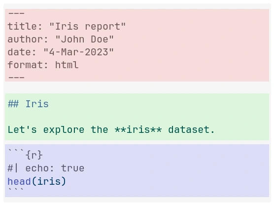
Create a Quarto document by creating a text file with .qmd extension. In RStudio, go to File > New File > Quarto Document. You are given the option to set title, author etc as well as output format. Set the output format as html. This document that you are working in is a Quarto notebook or R notebook. You can set the display mode to be Source or Visual (where text formatting is shown).
A Quarto file usually consists of a YAML header, text in markdown format and if needed some code in code chunks. All of these are optional. An empty qmd file is a valid Quarto file which will render to produce a blank html document.
1.1 YAML
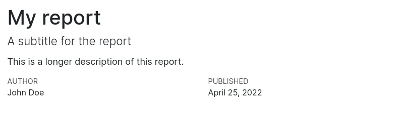
The content on the top of the Quarto document within three dashes is the YAML front matter. This is optional. It is really up to the author to decide how much information needs to be entered here. Here are some common base level YAML parameters.
---
title: "My report"
subtitle: "A subtitle for the report"
description: "This is a longer description of this report."
author: "John Doe"
date: "25-Apr-2022"
---
The default output format is HTML and this can be changed or arguments for this can be adjusted by specifying this in the YAML. Here is an updated version:
---
title: "My report"
subtitle: "A subtitle for the report"
description: "This is a longer description of this report."
author: "John Doe"
date: last-modified
date-format: "DD-MMM-YYYY"
format:
  html:
    toc: true
    toc-depth: 4
    number-sections: true
    number-depth: 4
---

# Section 1

This is some text

# Section 2

Here is some more text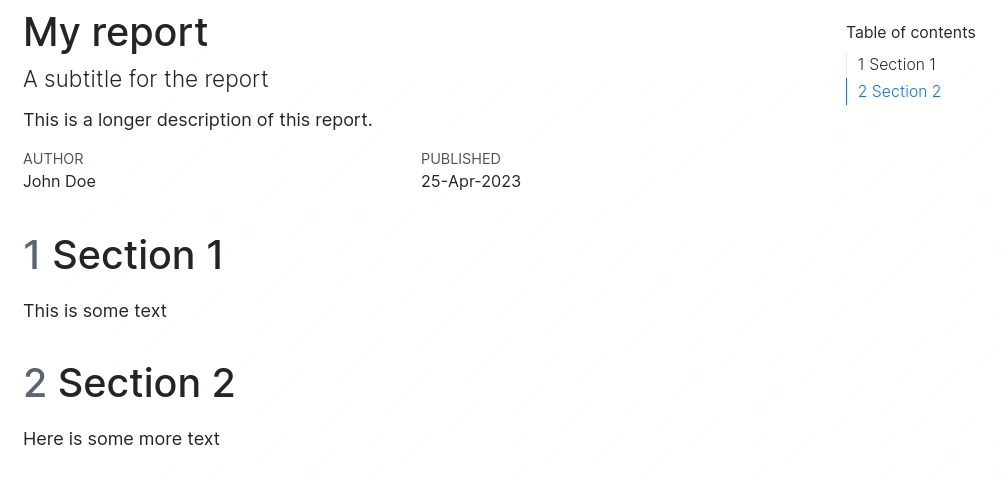
Date is now set as last-modified which means it is automatically updated whenever the document is rendered. The date format is adjusted by setting date-format: “DD-MMM-YYYY”. In addition, the output format is now explicitly specified. The table of contents is enabled and it’s depth is set to 4. Section numbering is enabled and depth is set to 4. Try changing some of these arguments to see how it affects the output.
Here is a more complex version:
---
title: "My report"
subtitle: "A subtitle for the report"
description: "This is a longer description of this report."
author: "John Doe"
date: last-modified
date-format: "DD-MMM-YYYY"
format:
  html:
    title-block-banner: true
    smooth-scroll: true
    toc: true
    toc-depth: 4
    toc-location: right
    number-sections: true
    number-depth: 4
    code-fold: true
    code-tools: true
    code-copy: true
    code-overflow: wrap
    df-print: kable
    standalone: false
    fig-align: left
---

# Section 1

This is some text

# Section 2

Here is some more text

```{r}
date()
```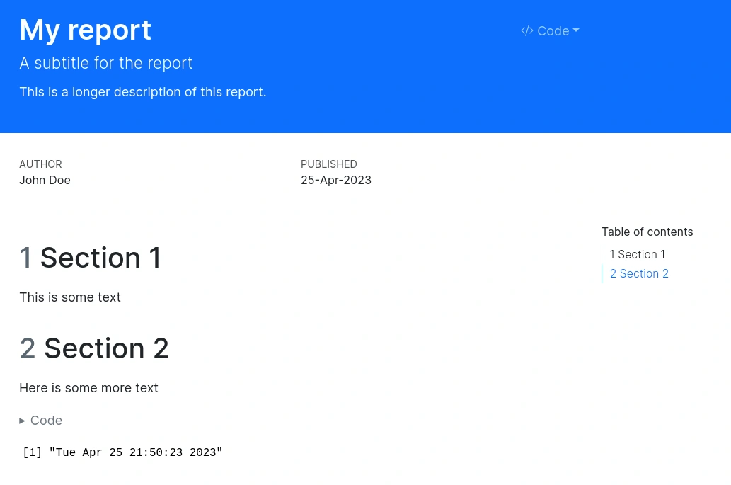
- title-block-banner: true Displays the blue banner
- code-fold: true Folds the code and reduces clutter
- code-copy: true Adds a copy icon in the code chunk and allows the code to be copied easily
- code-tools: true Adds options to the top right of the document to allow the user to show/hide all code chunks and view source code
- df-print: kable Sets the default method of displaying tables
- standalone: false Keeps dependencies as external files. When set to
true, Quarto tries to embed as many dependencies as possible into the output HTML file. Standalone documents may not always work with complex HTML files such as those with interactive graphics.
For a complete guide to YAML metadata for HTML, see here.
1.2 Markdown text
Markdown is a markup language similar to HTML, but simple and human-readable. There exists several variants of markdown with slight differences. Quarto uses Pandoc flavored markdown.
Headings are specified as such:
## Level 2 heading
### Level 3 heading
#### Level 4 heading
##### Level 5 heading
###### Level 6 heading
This *italic text* becomes italic text.
This **bold text** becomes bold text.
Subscript written like this H~2~O renders as H2O.
Superscript written like this 2^10^ renders as 210.
Bullet points are usually specified using -
- Point one
- Point two- Point one
- Point two
Block quotes can be specified using >.
> This is a block quote. This
> paragraph has two lines.
This is a block quote. This paragraph has two lines.
Lists can also be created inside block quotes.
> 1. This is a list inside a block quote.
> 2. Second item.
- This is a list inside a block quote.
- Second item.
Links can be created using [this](https://quarto.org) which renders like this.
1.3 Images
Images can be displayed from a relative local location or a full URL using 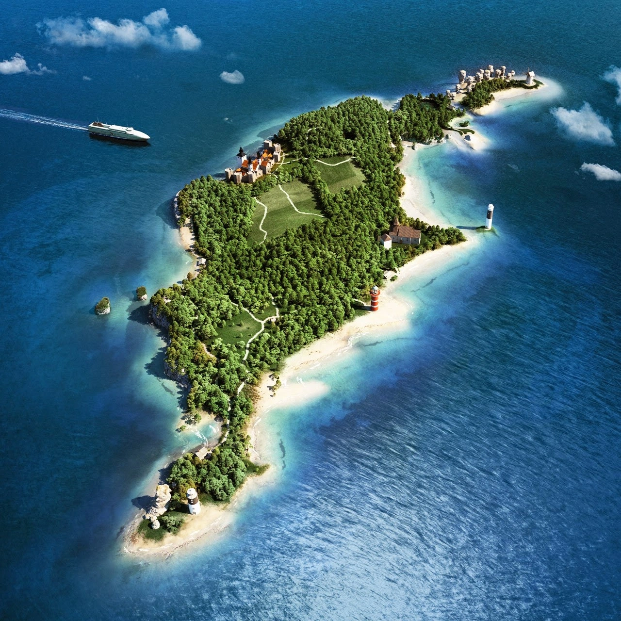. For example:

By default, the image is displayed at full scale or until it fills the display width. The image dimension can be adjusted {width=40%}.
For finer control, raw HTML can be used. For example;
<img src="assets/gotland.webp" width="150px">
Note
Using raw HTML would only work if the output format is an HTML format.
Images can also be displayed using R code.
This image is displayed at a size of 200 pixels.
```{r}
#| out-width: "200px"
knitr::include_graphics("assets/gotland.webp")
```
This image is displayed at a size of 75 pixels.
```{r}
#| out-width: "75px"
knitr::include_graphics("assets/gotland.webp")
```
1.4 Code
Text can be formatted as code. Code is displayed using monospaced font. Code formatting that stands by itself as a paragraph is called block code. Block codes are specified using three backticks ``` followed by code and then three more backticks.
This text below
```
This is generic block code.
```
renders like this
This is generic block code.Code formatting can also be included in the middle of a sentence. This is called inline code formatting. Using this `This is an inline formatted code.` renders like this: This is an inline formatted code.
The above codes are not actually executed. They are just text formatted in a different font. Code can be executed by specifying the language along with the backticks. Block code formatted as such:
```{r}
str(iris)
```
renders like this:
str(iris)'data.frame': 150 obs. of 5 variables:
$ Sepal.Length: num 5.1 4.9 4.7 4.6 5 5.4 4.6 5 4.4 4.9 ...
$ Sepal.Width : num 3.5 3 3.2 3.1 3.6 3.9 3.4 3.4 2.9 3.1 ...
$ Petal.Length: num 1.4 1.4 1.3 1.5 1.4 1.7 1.4 1.5 1.4 1.5 ...
$ Petal.Width : num 0.2 0.2 0.2 0.2 0.2 0.4 0.3 0.2 0.2 0.1 ...
$ Species : Factor w/ 3 levels "setosa","versicolor",..: 1 1 1 1 1 1 1 1 1 1 ...Code blocks are called chunks. The chunk is executed when this document is rendered. In the above example, the rendered output has two chunks; input and output chunks. The rendered code output is also given code highlighting based on the language. For example;
This code chunk
```{r}
#| eval: false
ggplot(dfr4,aes(x=Month,y=fraction,colour=Year,group=Year))+
  geom_point(size=2)+
  geom_line()+
  labs(x="Month",y="Fraction of support issues")+
  scale_colour_manual(values=c("#000000","#E69F00","#56B4E9",
  "#009E73","#F0E442","#006699","#D55E00","#CC79A7"))+
  theme_bw(base_size=12,base_family="Gidole")+
  theme(panel.border=element_blank(),
        panel.grid.minor=element_blank(),
        panel.grid.major.x=element_blank(),
        axis.ticks=element_blank())
```
when rendered (echo: true by default, but not evaluated) looks like
ggplot(dfr4, aes(x = Month, y = fraction, colour = Year, group = Year)) +
  geom_point(size = 2) +
  geom_line() +
  labs(x = "Month", y = "Fraction of support issues") +
  scale_colour_manual(values = c(
    "#000000", "#E69F00", "#56B4E9",
    "#009E73", "#F0E442", "#006699", "#D55E00", "#CC79A7"
  )) +
  theme_bw(base_size = 12, base_family = "Gidole") +
  theme(
    panel.border = element_blank(),
    panel.grid.minor = element_blank(),
    panel.grid.major.x = element_blank(),
    axis.ticks = element_blank()
  )
The behaviour of code chunks can be adjusted using chunk parameters or execution options. The chunk has several options which can be used to control chunk properties.
Using eval: false prevents that chunk from being executed. eval: true which is the default, executes the chunk. Using echo: false prevents the code from that chunk from being displayed. Using output: false hides the output from that chunk. Here are some of them:
| Option | Default | Description |
|---|---|---|
| eval | true | Evaluates the code in this chunk |
| echo | true | Display the code |
| output | true | true, false or asis |
| warning | true | Display warnings from code execution |
| error | false | Display error from code execution |
| message | true | Display messages from this chunk |
| include | true | Use false to hide code, output, messages and warnings |
Chunk options are specified like this:
```{r}
#| eval: false
#| echo: false
#| fig-height: 6
#| fig-width: 7
```
These chunk arguments or execution options can also be set globally in the YAML front matter.
---
execute:
  eval: true
  echo: false
---
There are many other execution options.
1.5 Tables
This is a table with a label and a dynamically generated caption.
```{r}
#| label: tbl-iris
#| tbl-cap: !expr paste0("The column names are ",paste(colnames(iris),collapse=", "))

head(iris)
```| Sepal.Length | Sepal.Width | Petal.Length | Petal.Width | Species |
|---|---|---|---|---|
| 5.1 | 3.5 | 1.4 | 0.2 | setosa |
| 4.9 | 3.0 | 1.4 | 0.2 | setosa |
| 4.7 | 3.2 | 1.3 | 0.2 | setosa |
| 4.6 | 3.1 | 1.5 | 0.2 | setosa |
| 5.0 | 3.6 | 1.4 | 0.2 | setosa |
| 5.4 | 3.9 | 1.7 | 0.4 | setosa |
Tables can be also be simple markdown.
|#|Sepal.Length|Sepal.Width|Petal.Length|Petal.Width|Species|
|---|---|---|---|---|---|
|1|5.1|3.5|1.4|0.2|setosa|
|2|4.9|3.0|1.4|0.2|setosa|
|3|4.7|3.2|1.3|0.2|setosa|
|4|4.6|3.1|1.5|0.2|setosa|

: This is a caption {#tbl-markdown-table}| # | Sepal.Length | Sepal.Width | Petal.Length | Petal.Width | Species |
|---|---|---|---|---|---|
| 1 | 5.1 | 3.5 | 1.4 | 0.2 | setosa |
| 2 | 4.9 | 3.0 | 1.4 | 0.2 | setosa |
| 3 | 4.7 | 3.2 | 1.3 | 0.2 | setosa |
| 4 | 4.6 | 3.1 | 1.5 | 0.2 | setosa |
1.6 Plots
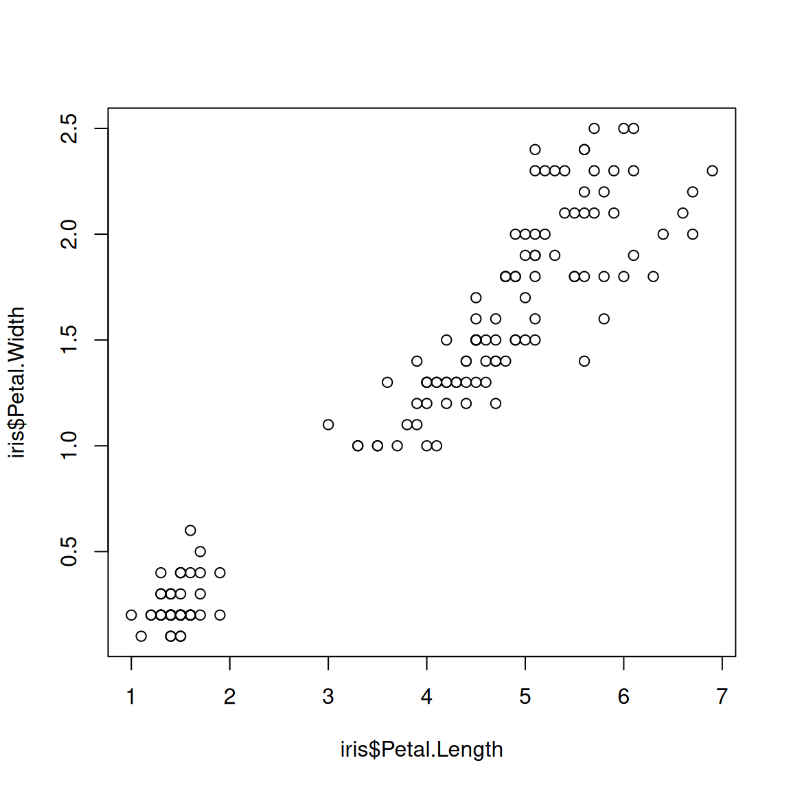
R Plots can be plotted like below:
```{r}
#| label: fig-plot-a
#| fig-cap: This is a figure caption.
#| fig-height: 6
#| fig-width: 6
plot(x=iris$Petal.Length,y=iris$Petal.Width)
```
1.7 Export
The Quarto notebook can be exported into various format. The most common formats are HTML and PDF.
1.7.1 HTML
The Quarto document can be previewed as an HTML inside RStudio by clicking the ‘Render’ button.
The document can be exported from R using the quarto R package.
quarto::quarto_render("document.qmd")The document can be rendered from the terminal as such:
quarto render document.qmdHTML documents can be opened and viewed in any standard browser such as Chrome, Safari, Firefox etc.
1.7.2 PDF
A qmd document can be converted to a PDF. Behind the scenes, the markdown is converted to TeX format. The conversion to PDF needs a tool that understands TeX format and converts to PDF. This can be tools like ‘MacTeX’, ‘MikTeX’ etc. which needs to be installed on the system. A light-weight option is to install tinytex through Quarto.
quarto install tinytexThe format argument in the YAML front matter must be changed to pdf.
Sometimes TeX converters may need additional libraries which may need to be installed. And all features of HTML are not supported on TeX which may return errors.
See here for more PDF options.
An alternative to using TeX based PDF generation is to use Typst. Quarto supports the Typst engine natively. More information about using Typst can be found in the Quarto typst documentation.
2 Report
In this example, we will recreate the parameterized report shown below:
The source code for the page is available on the page by clicking the code-tools icon on top right.
The aim of the report is to subset the iris dataset and create a report on the subsetted data. This is a parameterized report because the species to subset is provided as a parameter to the document during run time.
This is how the YAML metadata is organized:
---
title: '`{r} paste0(params$name," report")`'
subtitle: "Parameterized report"
author: "John Doe"
date: last-modified
format:
  html:
    title-block-banner: true
    toc: true
    number-sections: true
    code-tools: true
    fig-align: left

params:
  name: setosa
---- Since this a parameterized report,
paramsis defined in the YAML metadata. Parameters have to be defined with defaults. Here we have one parameternamewith default value setosa. A different argument to the parameter can be passed in while rendering the document. If no parameter is passed, the default value is used. - The title takes this parameter to create a title with the name.
- The output format is set to
html. - Table of contents (
toc) is enabled. title-block-banneris enabledcode-toolscreates a widget on the top right side of the document to view source code.
A heading is created through code using param value.
```{r}
#| echo: false
#| output: asis
cat("## ",params$name)
```
This code chunk is used to subset the iris dataset and display the first few rows of the subsetted data. The table has a label and a caption which is generated dynamically using the parameter value.
```{r}
#| label: tbl-data
#| tbl-cap: !expr paste0("Data for ",params$name," species.")
iris_filtered <- subset(iris, iris$Species == params$name)
head(iris_filtered)
```- It is important that the table label starts with
tbl- - The table caption is generated from code using the special
!exprusage
This code chunk is used to create a plot along with plot caption and plot numbering.
```{r}
#| label: fig-scatterplot
#| fig-cap: !expr paste0("Scatterplot of ",params$name," species.")
ggplot(iris_filtered,aes(Sepal.Length,Petal.Length,col=Species))+
    geom_point()+
    labs(title=params$name)
```- It is important that the figure label starts with
fig- - The figure caption is generated from code using the special
!exprusage
In the last chunk, an image of the species is displayed.
```{r}
#| echo: false
#| label: fig-species
#| fig-cap: !expr paste0("Photograph of ",params$name," species.")

imgs <- c(
    "setosa" = "assets/setosa.jpg",
    "versicolor" = "assets/versicolor.jpg",
    "virginica" = "assets/virginica.jpg"
)

knitr::include_graphics(imgs[[params$name]])
```
Cross-references to the table and figure can be created using @tbl-data and @fig-scatterplot respectively.
A parameterized report can be rendered from the terminal as such:
quarto render report.qmd -P name:versicolorAlternatively, the parameters can be provided in a separate YAML file and passed in as such:
quarto render report.qmd --execute-params params.yamlLastly, the parameter can be passed in from R as such:
quarto::quarto_render("report.qmd", execute_params = list(name = "versicolor"))Tasks
- Try to create a new report for the species versicolor
- Try to convert the document to PDF using Latex (
format: pdf) and Typst (format: typst)
HTML outputs are documented here.
TipTroubleshooting
- YAML is indentation-sensitive. If rendering fails before any code runs, check for missing spaces, tabs or unmatched quotes in the YAML front matter.
- If R reports that a package is missing, install it with
install.packages("package-name")and render again. - If an image does not appear, check that the file path is relative to the
.qmdfile and that the file name matches exactly. - If a table or figure cross-reference does not work, check that the chunk label starts with
tbl-orfig-and is unique in the document. - If PDF rendering fails, try HTML first. PDF output may require TinyTeX or another TeX installation, and some HTML-specific features may not convert cleanly.
3 RevealJS
Now, we will convert the report to a presentation using revealjs.
The raw code is available here.
- The most important change is
format: htmltoformat: revealjs - Slides are defined by heading
## - Slides can be hidden using
{visibility="hidden"}
## Title {visibility="hidden"}- Incremental lists can be created like this
::: {.incremental}
- Eat spaghetti
- Drink wine
:::- Columns can be defined like this
:::: {.columns}

::: {.column width="50%"}
Left column
:::

::: {.column width="50%"}
Right column
:::

::::- Speaker notes are created like this:
::: {.notes}
Speaker notes go here.
:::
The presenter view is enabled by pressing the S key.
- The presentation theme can be changed
format:
  revealjs:
theme: dark- Minor slide content can be defined as below. This content will be smaller font size and pushed to the bottom.
::: aside
Some additional commentary of more peripheral interest.
:::- Code chunks can have line highlighting
```{r}
#| code-line-numbers: "4-5"
library(ggplot2)

ggplot(iris,aes(Sepal.Length, Petal.Length))+
  geom_point()+
  theme_bw()
```- Tabset panels
::: {.panel-tabset}

### Tab A

Content for `Tab A`

### Tab B

Content for `Tab B`

:::
RevealJS features are documented here.
4 Projects
So far, the output formats have been a single document. We can also have a project composed of multiple documents and document types. In this case, the files are organised in a directory and the configuration is defined in _quarto.yml. This will be referred to as the config file. Think of this as a shared YAML metadata file for all of the documents. In addition, an index.qmd file defines the home page.
For a website, the minimal config looks like this
project:
  type: website
And for a book:
project:
  type: book
Then running quarto render renders the output into a directory named _site. During development, quarto preview starts a local preview server and updates the site as files change. The output can be changed, for example, to docs for GitHub Pages.
project:
  type: website
  output-dir: docs
The output format by default is HTML. This can be changed or modified by adding format to the config file or to individual qmd files. The parameters defined in the config file will be shared by all other qmd files.
To create a project in RStudio, go to File > New Project, then select directory and then a project type such as website, blog or book. Try creating one based on what interests you. Website and blog documentation is here and books are here.
For more project options, see here. To build your own personal website, see the topic quarto-site in the list of labs.
5 Session
Click here
sessionInfo()R version 4.5.3 (2026-03-11)
Platform: x86_64-conda-linux-gnu
Running under: Ubuntu 26.04 LTS
Matrix products: default
BLAS/LAPACK: /home/roy/miniforge3/envs/r-4.5/lib/libopenblasp-r0.3.33.so; LAPACK version 3.12.0
locale:
[1] LC_CTYPE=en_US.UTF-8 LC_NUMERIC=C
[3] LC_TIME=en_US.UTF-8 LC_COLLATE=en_US.UTF-8
[5] LC_MONETARY=en_US.UTF-8 LC_MESSAGES=en_US.UTF-8
[7] LC_PAPER=en_US.UTF-8 LC_NAME=C
[9] LC_ADDRESS=C LC_TELEPHONE=C
[11] LC_MEASUREMENT=en_US.UTF-8 LC_IDENTIFICATION=C
time zone: Europe/Stockholm
tzcode source: system (glibc)
attached base packages:
[1] stats graphics grDevices utils datasets methods base
other attached packages:
[1] knitr_1.51 stringr_1.6.0 dplyr_1.2.1 ggplot2_4.0.3
loaded via a namespace (and not attached):
[1] vctrs_0.7.3 cli_3.6.6 rlang_1.2.0 xfun_0.59
[5] stringi_1.8.7 otel_0.2.0 generics_0.1.4 S7_0.2.2
[9] jsonlite_2.0.0 glue_1.8.1 htmltools_0.5.9 scales_1.4.0
[13] rmarkdown_2.31 grid_4.5.3 tibble_3.3.1 evaluate_1.0.5
[17] fastmap_1.2.0 yaml_2.3.12 lifecycle_1.0.5 compiler_4.5.3
[21] RColorBrewer_1.1-3 pkgconfig_2.0.3 htmlwidgets_1.6.4 farver_2.1.2
[25] digest_0.6.39 R6_2.6.1 tidyselect_1.2.1 pillar_1.11.1
[29] magrittr_2.0.5 withr_3.0.3 tools_4.5.3 gtable_0.3.6