Neural Networks

1 Introduction

In this live coding session we will implement a vanilla autoencoder – a specific neural network architecture. We will be using keras interface to tensorflow which is a neural net engine.

Autoencoders can be used in different contexts, from watermark removal to semantic segmentation of images. We will use our autoencoder to reduce dimensionality of the input data: 5000 SNPs per individual coming from the HapMap3 project. This is a toy dataset distilled from the original HapMap3 data for teaching purposes and computational tractability.

The goal is to visually compare autoencoder dimensionality reduction to classical PCA.

1.1 Load packages

library(keras3)
library(tidyverse)
library(ggplot2)

1.2 Loading the data

load("assets/vanilla_autoencoder.Rd")

1.3 Scaling SNP dosage

x_train <- as.matrix(orig_geno) / 2

1.4 Traditional PCA

pca_res <- prcomp(x_train, rank. = 2)
pca_data <- as.data.frame(pca_res$x)
pca_data <- cbind(pca_data, orig_pheno)

ggplot(pca_data, aes(x = PC1, y = PC2, color = Population)) +
  geom_point(alpha = 0.7, size = 2) +
  theme_minimal() +
  labs(title = "PCA Embedding of Populations",
       x = "PC1", y = "PC2")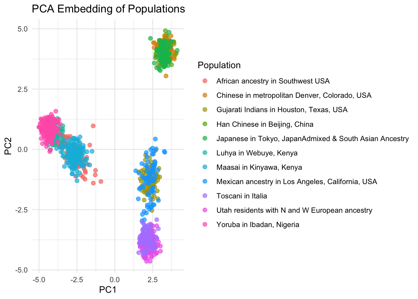

2 Autoencoder

First, we need to specify the input dimensions, in our case, the number of variables-SNPs and the desired dimensionality of the latent space. We choose 2 dimensions to easily plot them on screen.

input_dim <- ncol(x_train)
latent_dim <- 2

2.1 Encoder

encoder <- keras_model_sequential(name = "encoder") |>
  layer_dense(256, activation = "relu", input_shape = input_dim) |>
  layer_dense(128, activation = "relu") |>
  layer_dense(latent_dim)

2.2 Decoder

decoder <- keras_model_sequential(name = "decoder") |>
  layer_dense(128, activation = "relu", input_shape = latent_dim) |>
  layer_dense(256, activation = "relu") |>
  layer_dense(input_dim)

2.3 Autoencoder

We now combine the encoder and the decoder

autoencoder <- keras_model_sequential(layers=list(encoder, decoder), name = "autoencoder")

And to make sure all is as expected, we visualise our architecture:

plot(autoencoder, show_layer_names = TRUE, show_shapes = TRUE, expand_nested = TRUE)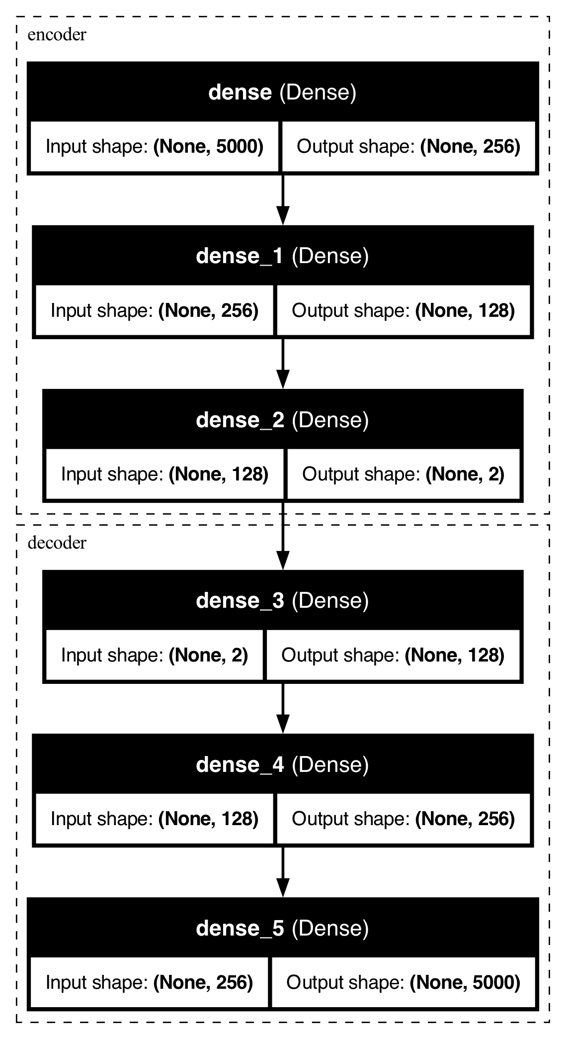

If everything seems to be fine, we can compile the model.

2.4 Compile model

autoencoder |> compile(
  optimizer = optimizer_adam(),
  loss = loss_mean_squared_error
)

2.5 Training

history <- autoencoder |> fit(
  x = x_train,
  y = x_train,
  epochs = 50,
  batch_size = 32,
  validation_split = 0.2,
  shuffle = TRUE
)

plot(history)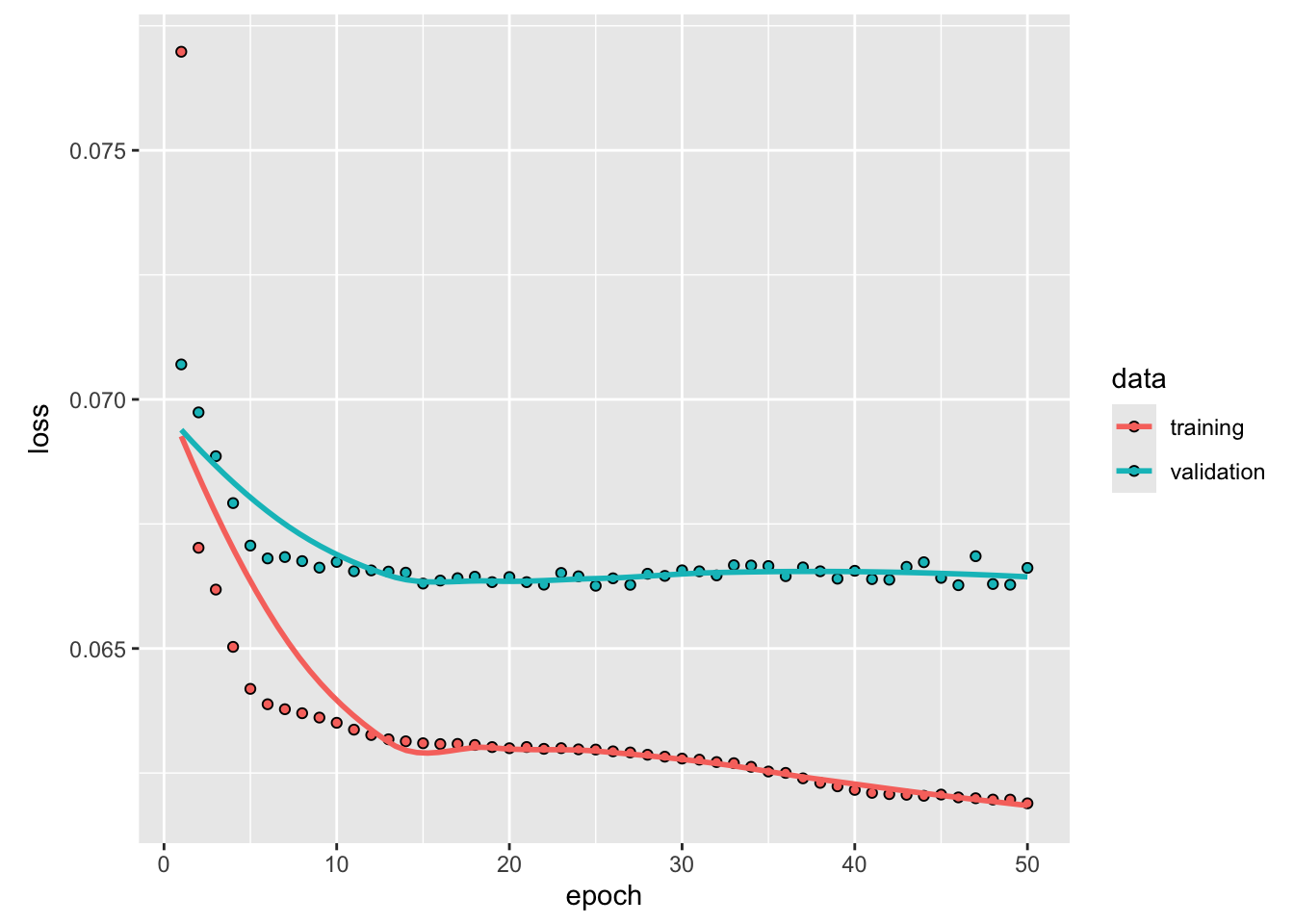

Finally, we are ready to visualise the latent space.

2.6 Latent space visualization

latent <- predict(encoder, x_train)

scores <- as.data.frame(latent)
colnames(scores) <- c("Z1", "Z2")

scores$Population <- orig_pheno$Population

ggplot(scores, aes(Z1, Z2, colour = Population)) +
  geom_point(size = 2) +
  theme_classic() +
  ggsci::scale_color_d3("category20")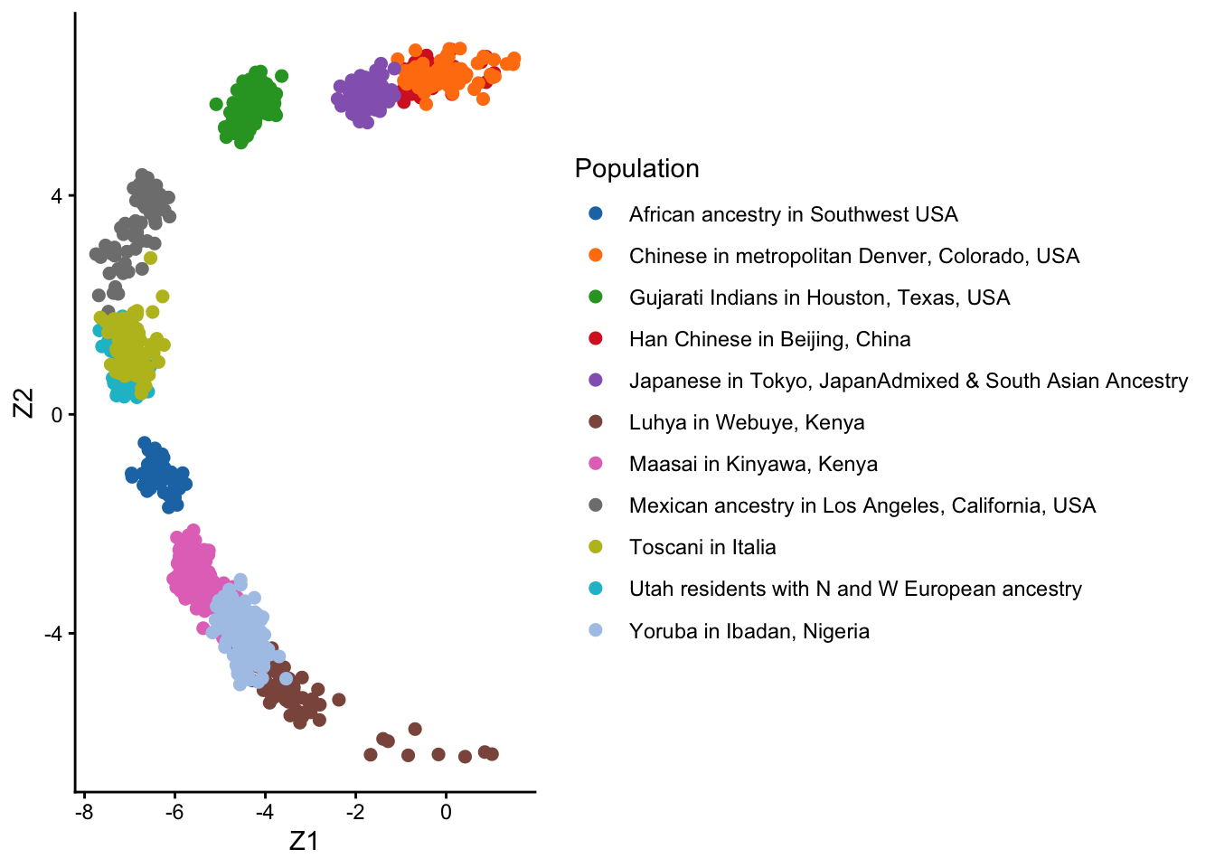

37/37 - 0s - 871us/step

We can also compute the mean reconstruction MSE.

x_recon <- predict(autoencoder, x_train)
mean((x_train - x_recon)^2)

37/37 - 0s - 1ms/step
[1] 0.06260577

3 Session

Click here

sessionInfo()

R version 4.6.0 (2026-04-24)
Platform: aarch64-apple-darwin23
Running under: macOS Tahoe 26.5.2

Matrix products: default
BLAS:   /Library/Frameworks/R.framework/Versions/4.6/Resources/lib/libRblas.0.dylib 
LAPACK: /Library/Frameworks/R.framework/Versions/4.6/Resources/lib/libRlapack.dylib;  LAPACK version 3.12.1

locale:
[1] en_US.UTF-8/en_US.UTF-8/en_US.UTF-8/C/en_US.UTF-8/en_US.UTF-8

time zone: Europe/Stockholm
tzcode source: internal

attached base packages:
[1] stats     graphics  grDevices utils     datasets  methods   base     

other attached packages:
 [1] lubridate_1.9.5 forcats_1.0.1   stringr_1.6.0   dplyr_1.2.1    
 [5] purrr_1.2.2     readr_2.2.0     tidyr_1.3.2     tibble_3.3.1   
 [9] ggplot2_4.0.3   tidyverse_2.0.0 keras3_1.5.1   

loaded via a namespace (and not attached):
 [1] generics_0.1.4     stringi_1.8.9      lattice_0.22-9     hms_1.1.4         
 [5] digest_0.6.39      magrittr_2.0.5     timechange_0.4.0   evaluate_1.0.5    
 [9] grid_4.6.0         RColorBrewer_1.1-3 fastmap_1.2.0      rprojroot_2.1.1   
[13] jsonlite_2.0.0     Matrix_1.7-5       whisker_0.4.1      tfruns_1.5.4      
[17] mgcv_1.9-4         tensorflow_2.20.0  scales_1.4.0       codetools_0.2-20  
[21] cli_3.6.6          rlang_1.3.0        splines_4.6.0      base64enc_0.1-6   
[25] withr_3.0.3        yaml_2.3.12        otel_0.2.0         tools_4.6.0       
[29] tzdb_0.5.0         zeallot_0.2.0      here_1.0.2         reticulate_1.46.0 
[33] vctrs_0.7.3        R6_2.6.1           png_0.1-9          lifecycle_1.0.5   
[37] htmlwidgets_1.6.4  pkgconfig_2.0.3    pillar_1.11.1      gtable_0.3.6      
[41] glue_1.8.1         Rcpp_1.1.2         xfun_0.60          tidyselect_1.2.1  
[45] knitr_1.51         farver_2.1.2       nlme_3.1-169       htmltools_0.5.9   
[49] ggsci_5.2.0        labeling_0.4.3     rmarkdown_2.31     dotty_0.1.0       
[53] compiler_4.6.0     S7_0.2.2