data.table

RaukR 2026 • Data Science With R

Fast, memory-efficient tabular data wrangling in R, compared with base R and the tidyverse.
Author

Markus Mayrhofer

Published

18-Aug-2026

NoteCoding exercise

We recommend that you run the code sections as you work through this exercise. You can copy-paste into a Quarto or R script and run line by line using .

library(data.table)   # the topic of this lab
library(dplyr)        # tidyverse reference implementations
library(readr)        # read_tsv(), for the file-reading benchmark
library(bench)        # benchmarking
library(ggplot2)      # benchmark plots
theme_set(theme_minimal())

# data.table is multi-threaded and picks a sensible number of threads by default
# (half the logical CPUs). getDTthreads() reports what it will use.
getDTthreads()
[1] 5

1 Introduction

data.table is an R package for working with rectangular / tabular data: rows are observations, columns are variables, each cell is one value. Most data-wrangling tasks are combinations of four basic actions:

Question Operation
Which rows do I keep? filter rows
Which columns do I keep or compute? select / mutate columns
Should I calculate separately for each group? group by
Do I need information from another table? join

Where it comes from. data.table was created by Matt Dowle, with version 1.0 on CRAN in April 2006, and was long co-developed with Arun Srinivasan. It is now maintained by a wider team (Tyson Barrett is the current CRAN maintainer, with Jan Gorecki, Michael Chirico, Toby Hocking and others). It grew out of a practical problem: row-wise operations on a base R data.frame – filtering, rbind, merge – rebuild every column, which becomes slow and memory-hungry once tables get large. data.table is written largely in C, is multi-threaded, adds or changes columns by reference (without copying), and ships with fast file readers (fread / fwrite). It keeps a deliberately small dependency footprint – just base R – which is part of why it stays fast and stable. The cost is a terse, bracket-based syntax, which this lab unpacks.

In this lab we express each of these in three styles and compare them:

  • base R: the tools that ship with R ([, $, subset(), tapply(), aggregate(), merge()).
  • tidyverse (dplyr): a sequence of named verbs joined by the pipe |>. Shown here only for comparison; many of you will already know it.
  • data.table: the focus of today. Everything happens inside DT[i, j, by].
NoteThe one idea to remember: DT[i, j, by]
DT[ i ,  j ,  by ]
|  |    |    `-- group by these columns
|  |    `------- compute, select, or update columns
|  `------------ keep or match these rows
`--------------- the data.table object

Read it as: take rows i, do j, separately within each by group. If there is no grouping, leave by out. If there is no row filter, leave i empty but keep the comma: DT[, j].

Two shorthands appear constantly:

  • .N = number of rows in the current group (like dplyr::n()).
  • .() = shorthand for list(); used in j to return or name columns.

2 Data: a simulated genotyping cohort

We simulate genetic data because it produces large tables, which is exactly where data.table earns its keep. No files to download: the generator below is fully reproducible. The biological terms are only labels; the same row/column/group/join ideas apply to any large table.

Term Meaning here
sample one person or specimen
variant one genomic position where samples may differ
genotype number of alternate copies: 0, 1, or 2; -1 means missing
read depth how many sequencing reads cover a site
genotype quality confidence score for the genotype call
allele frequency average alternate-copy frequency across samples

The data has three linked tables:

  • samples: one row per sample (population, sex, batch, case/control).
  • variants: one row per variant (chromosome, position, gene, consequence, frequency).
  • genotypes: one row per sample x variant pair (genotype, read depth, quality). This is the tall table.
Run to generate the data – click to expand
simulate_genotyping <- function(n_samples = 500, n_variants = 4000, seed = 42) {
  set.seed(seed)

  # samples: one row per sample
  pops <- c("AFR", "AMR", "EAS", "EUR", "SAS")
  samples <- data.table(
    sample_id  = sprintf("S%05d", seq_len(n_samples)),
    population = sample(pops, n_samples, replace = TRUE,
                        prob = c(0.22, 0.14, 0.20, 0.30, 0.14)),
    sex        = sample(c("M", "F"), n_samples, replace = TRUE),
    batch      = sample(sprintf("batch%02d", 1:8), n_samples, replace = TRUE),
    phenotype  = rbinom(n_samples, 1, 0.35)   # 1 = case, 0 = control
  )

  # variants: one row per variant
  chroms <- c(1:22, "X")
  conseq <- c("synonymous", "missense", "stop_gained", "splice_region", "intron", "UTR")
  variants <- data.table(
    variant_id  = sprintf("rs%07d", seq_len(n_variants)),
    chrom       = sample(chroms, n_variants, replace = TRUE),
    pos         = sample(1e6:2.5e8, n_variants, replace = TRUE),
    ref         = sample(c("A", "C", "G", "T"), n_variants, replace = TRUE),
    alt         = sample(c("A", "C", "G", "T"), n_variants, replace = TRUE),
    gene        = sprintf("GENE%04d", sample(1:1500, n_variants, replace = TRUE)),
    consequence = sample(conseq, n_variants, replace = TRUE,
                         prob = c(0.30, 0.25, 0.03, 0.07, 0.25, 0.10)),
    maf         = round(rbeta(n_variants, 0.6, 6), 4)   # skewed toward rare
  )
  flip <- variants$alt == variants$ref
  variants[flip, alt := fifelse(ref == "A", "G", "A")]

  # genotypes: one row per sample x variant (the tall table)
  geno <- CJ(sample_id = samples$sample_id, variant_id = variants$variant_id)
  geno[variants, maf := i.maf, on = "variant_id"]
  n <- nrow(geno)
  p <- geno$maf
  u <- runif(n)
  geno[, genotype := fifelse(u < (1 - p)^2, 0L,
                       fifelse(u < (1 - p)^2 + 2 * p * (1 - p), 1L, 2L))]
  geno[runif(n) < 0.02, genotype := -1L]                # 2% missing
  geno[, read_depth       := rpois(n, lambda = 30)]
  geno[, genotype_quality := pmin(99L, rpois(n, lambda = 45))]
  geno[, maf := NULL]
  setcolorder(geno, c("sample_id", "variant_id", "genotype", "read_depth", "genotype_quality"))

  list(genotypes = geno[], variants = variants[], samples = samples[])
}

dat       <- simulate_genotyping(n_samples = 500, n_variants = 4000, seed = 42)
genotypes <- dat$genotypes
variants  <- dat$variants
samples   <- dat$samples

# Plain data.frame copies. The base R *and* tidyverse code below both use these,
# so each style is measured on its own native input: base R indexing on a
# data.frame, dplyr verbs on a data.frame, and data.table's `[` on a data.table.
genotypes_df <- as.data.frame(genotypes)
variants_df  <- as.data.frame(variants)
samples_df   <- as.data.frame(samples)

dim(genotypes)                                  # 500 x 4000 = 2,000,000 rows
format(object.size(genotypes), units = "MB")
head(genotypes, 4)
[1] 2000000       5
[1] "53.7 Mb"
sample_id variant_id genotype read_depth genotype_quality
S00001 rs0000001 0 27 48
S00001 rs0000002 0 25 53
S00001 rs0000003 1 33 43
S00001 rs0000004 0 27 44
Tip

Exactly 2,000,000 rows (500 samples x 4000 variants), the same on every machine because the seed is fixed. The size is intentional: small examples hide the memory and copying behaviour that matters in real analyses.

The data and every analysis result below – allele frequencies, call rates, gene counts – are identical wherever you run this. The benchmark numbers are not: times and memory allocations both depend on your hardware and package versions, and the ranking between the three styles can change with them.

3 Core operations

Each operation below is shown in all three styles. Watch where the row filter, the column calculation, and the grouping live in each.

NoteWhy the tidyverse code uses genotypes_df

data.table inherits from data.frame, so dplyr verbs do work on a data.table – but dplyr then has to convert it, which makes dplyr look slower and more memory-hungry than it really is. To keep the later benchmarks fair, the base R and tidyverse code both work on the plain data.frame copies (genotypes_df, variants_df, samples_df) while the data.table code works on the data.table. Each style is measured on its own native input.

A tibble would work equally well: it is a data.frame underneath and benchmarks within a few percent. Plain data.frame also keeps the printed results in the same style as the other two engines.

3.1 Filter rows

Get genotype rows where the genotype is a homozygous alternate call and read depth is adequate (showing top three).

# base R
head(genotypes_df[genotypes_df$genotype == 2 & genotypes_df$read_depth >= 20, ], 3)

# tidyverse
genotypes_df |> filter(genotype == 2, read_depth >= 20) |> head(3)

# data.table: the row condition goes in i, before the first comma
genotypes[genotype == 2 & read_depth >= 20][1:3]
sample_id variant_id genotype read_depth genotype_quality
30 S00001 rs0000030 2 30 51
159 S00001 rs0000159 2 25 41
166 S00001 rs0000166 2 30 38
sample_id variant_id genotype read_depth genotype_quality
S00001 rs0000030 2 30 51
S00001 rs0000159 2 25 41
S00001 rs0000166 2 30 38
sample_id variant_id genotype read_depth genotype_quality
S00001 rs0000030 2 30 51
S00001 rs0000159 2 25 41
S00001 rs0000166 2 30 38

Under the hood: all three build a TRUE/FALSE vector over the rows and keep the TRUE ones. All three return a new table – the original is untouched – so you pay memory for the rows you keep, and you would normally assign the result a name.

3.2 Select columns

# base R
head(variants_df[, c("variant_id", "gene", "maf")], 3)

# tidyverse
variants_df |> select(variant_id, gene, maf) |> head(3)

# data.table: selected columns go in j as .(...)
variants[, .(variant_id, gene, maf)][1:3]
variant_id gene maf
rs0000001 GENE1396 0.2884
rs0000002 GENE0574 0.0026
rs0000003 GENE1463 0.1125
variant_id gene maf
rs0000001 GENE1396 0.2884
rs0000002 GENE0574 0.0026
rs0000003 GENE1463 0.1125
variant_id gene maf
rs0000001 GENE1396 0.2884
rs0000002 GENE0574 0.0026
rs0000003 GENE1463 0.1125

Under the hood: all three return a new table object, but the data vectors themselves are not duplicated until something modifies them.

3.3 Add a column

# base R (shallow copy: the other columns are shared with variants_df)
v_tmp <- variants_df
v_tmp$is_rare <- v_tmp$maf < 0.01
head(v_tmp[, c("variant_id", "maf", "is_rare")], 3)

# tidyverse (returns a new object)
variants_df |> mutate(is_rare = maf < 0.01) |>
  select(variant_id, maf, is_rare) |> head(3)

# data.table: := adds/updates a column by reference (no copy)
variants[, is_rare := maf < 0.01]
variants[, .(variant_id, maf, is_rare)][1:3]
variant_id maf is_rare
rs0000001 0.2884 FALSE
rs0000002 0.0026 TRUE
rs0000003 0.1125 FALSE
variant_id maf is_rare
rs0000001 0.2884 FALSE
rs0000002 0.0026 TRUE
rs0000003 0.1125 FALSE
variant_id maf is_rare
rs0000001 0.2884 FALSE
rs0000002 0.0026 TRUE
rs0000003 0.1125 FALSE
WarningReference semantics

:= changes variants in place: there is no new object to assign, and every other reference to that table sees the change. Use copy(variants) first if you need an untouched snapshot. A function that receives a data.table and uses := can modify the caller’s object unless it copies internally.

The base R and tidyverse versions above are not expensive either: a data.frame is a list of columns, so they share the unchanged columns and duplicate only the column you touch. The copies that actually cost you are row-wise – filters, rbind, joins – which have to rebuild every column.

3.4 Group and summarise

For each sample, among called genotypes, compute the mean read depth and the number of called genotypes.

# base R (aggregate() returns a matrix column, so flatten and rename)
called <- genotypes_df[genotypes_df$genotype >= 0, ]
agg <- aggregate(read_depth ~ sample_id, data = called,
                 FUN = function(x) c(mean_depth = mean(x), n_called = length(x)))
agg <- do.call(data.frame, agg)
names(agg) <- c("sample_id", "mean_depth", "n_called")
head(agg, 3)

# tidyverse
genotypes_df |>
  filter(genotype >= 0) |>
  group_by(sample_id) |>
  summarise(mean_depth = mean(read_depth), n_called = n()) |>
  head(3)

# data.table: i filters, j computes, by defines the groups
genotypes[genotype >= 0,
          .(mean_depth = mean(read_depth), n_called = .N),
          by = sample_id][1:3]
sample_id mean_depth n_called
S00001 30.13361 3907
S00002 30.05686 3922
S00003 29.79305 3914
sample_id mean_depth n_called
S00001 30.13361 3907
S00002 30.05686 3922
S00003 29.79305 3914
sample_id mean_depth n_called
S00001 30.13361 3907
S00002 30.05686 3922
S00003 29.79305 3914

3.5 Join tables

Attach each variant’s consequence and gene to the genotype rows, using variant_id as the shared key.

# base R (merge() reorders around the join key; re-sort to match the others)
m <- merge(genotypes_df, variants_df[, c("variant_id", "consequence", "gene")],
           by = "variant_id")
m <- m[order(m$sample_id, m$variant_id),
       c("sample_id", "variant_id", "genotype", "consequence", "gene")]
head(m, 3)

# tidyverse
genotypes_df |>
  inner_join(select(variants_df, variant_id, consequence, gene), by = "variant_id") |>
  select(sample_id, variant_id, genotype, consequence, gene) |>
  head(3)

# data.table: x[y, on = "key"]
variants[genotypes, on = "variant_id",
         .(sample_id, variant_id, genotype, consequence, gene)][1:3]
sample_id variant_id genotype consequence gene
1 S00001 rs0000001 0 synonymous GENE1396
975 S00001 rs0000002 0 intron GENE0574
1338 S00001 rs0000003 1 UTR GENE1463
sample_id variant_id genotype consequence gene
S00001 rs0000001 0 synonymous GENE1396
S00001 rs0000002 0 intron GENE0574
S00001 rs0000003 1 UTR GENE1463
sample_id variant_id genotype consequence gene
S00001 rs0000001 0 synonymous GENE1396
S00001 rs0000002 0 intron GENE0574
S00001 rs0000003 1 UTR GENE1463

4 Keys

The joins above used on = to match columns ad-hoc. If you look up or join on the same column repeatedly, it is worth setting a key.

A key is one or more columns that a data.table is physically sorted by. setkey(DT, col) reorders the rows of DT by col – in place, by reference – and records that order.

setkey(genotypes, sample_id)
key(genotypes)
[1] "sample_id"

Because the rows are now sorted by sample_id, data.table can find rows by binary search rather than scanning the whole table:

genotypes["S00001"][1:3]     # keyed lookup: one sample's rows, found directly
sample_id variant_id genotype read_depth genotype_quality
S00001 rs0000001 0 27 48
S00001 rs0000002 0 25 53
S00001 rs0000003 1 33 43

A key speeds up three things on the key column(s):

  • Row lookups, as above.
  • Repeated joins: two tables keyed on the same column join by a fast sorted merge.
  • Grouping by the key column.

You do not always need a key – the on = joins above work without one – but set a key when you will hit the same column many times, so the sort cost is paid once. setindex() gives a similar speed-up without physically re-ordering the table.

5 Benchmarks: time and memory

bench::mark() runs each expression and records elapsed time, memory allocated, and garbage collections. Time matters because slow code interrupts analysis. Memory matters because large tables can fail when R runs out of RAM. check = FALSE allows small differences in output shape between engines.

Helper: plot a bench::mark result (time, and memory when measured)
bench_fig <- function(b, engines) {
  cols <- c("#D55E00", "#0072B2", "#009E73")   # base_R, middle engine, data.table
  names(cols) <- engines

  long <- data.frame(engine = as.character(b$expression),
                     metric = "median time (ms)",
                     value  = as.numeric(b$median) * 1000)
  if (!is.null(b$mem_alloc) && !all(is.na(b$mem_alloc))) {
    long <- rbind(long, data.frame(
      engine = as.character(b$expression),
      metric = "memory allocated (MB)",
      value  = as.numeric(b$mem_alloc) / 1024^2))
  }
  # rev() so the first engine (base_R) sits on top after coord_flip
  long$engine <- factor(long$engine, levels = rev(engines))
  long$metric <- factor(long$metric,
                        levels = c("median time (ms)", "memory allocated (MB)"))

  # horizontal bars without coord_flip, so facet free scales work per panel
  ggplot(long, aes(x = value, y = engine, fill = engine)) +
    geom_col(width = 0.65, show.legend = FALSE, orientation = "y") +
    geom_text(aes(label = round(value, 1)), hjust = -0.15, size = 3.3) +
    facet_wrap(~ metric, scales = "free_x") +   # each metric gets its own value axis
    scale_fill_manual(values = cols) +
    scale_x_continuous(expand = expansion(mult = c(0, 0.18))) +
    labs(x = NULL, y = NULL) +
    theme_minimal(base_size = 12) +
    theme(panel.grid.major.y = element_blank())
}

5.1 Grouped aggregation: per-variant allele frequency

For each variant, among called genotypes, allele frequency is sum(genotype) / (2 * n_called).

bench_agg <- bench::mark(
  base_R = {
    ca <- genotypes_df[genotypes_df$genotype >= 0, c("variant_id", "genotype")]
    tapply(ca$genotype, ca$variant_id, sum) /
      (2 * tapply(ca$genotype, ca$variant_id, length))
  },
  tidyverse = genotypes_df |>
    filter(genotype >= 0) |>
    group_by(variant_id) |>
    summarise(af = sum(genotype) / (2 * n()), .groups = "drop"),
  data.table = genotypes[genotype >= 0,
                         .(af = sum(genotype) / (2 * .N)),
                         by = variant_id],
  check = FALSE,
  iterations = 3
)
bench_agg[, c("expression", "median", "mem_alloc", "n_gc")]
expression median mem_alloc
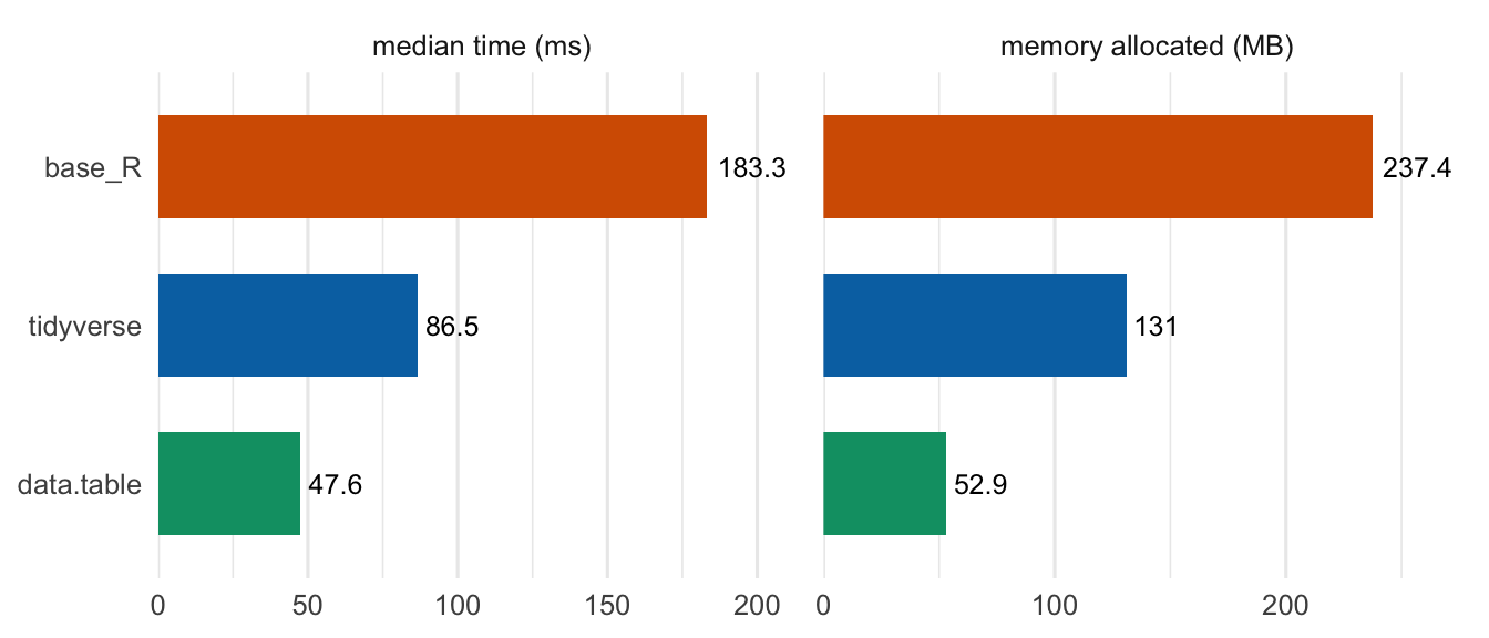
base_R 183.3ms 237.4MB
tidyverse 86.5ms 131MB
data.table 47.6ms 52.9MB
bench_fig(bench_agg, c("base_R", "tidyverse", "data.table"))
Figure 1: Grouped aggregation over 2,000,000 genotype rows: median run time and memory allocated, per engine. Lower is better.
NoteReading this result

The consistent, reproducible win here is memory: data.table allocates several times less than either alternative, because it groups without materialising large intermediate copies. If your table is big enough that RAM is the binding constraint, that difference decides whether the job runs at all.

Time is less stable. data.table spreads grouping across cores, while base R and dplyr do this work on a single core – so the time ranking depends on the machine: how many cores it has, how fast one core is, how many threads data.table is actually using (see getDTthreads() above), and which package versions are installed. Expect your own numbers to differ from those above, possibly in a different order.

That is why we measure rather than assert: which tool wins depends on the operation, the shape of the data, the hardware, and whether time or memory is scarce.

5.2 Three-table join

Attach variant consequence + gene and sample population to every genotype row.

WarningRead this benchmark with one caveat

The setkey() calls happen before bench::mark(), so the one-time cost of sorting the tables is not included in the data.table timing, while base R and dplyr pay their full cost inside the timed expression. That matches a real application – you sort once, then join and look up many times – but this benchmark performs only a single join. For a genuine one-off join you would have to add the sort cost to data.table’s time, reducing its advantage slightly.

# keyed joins are sorted-merge joins (fast); set keys once, outside the timing
setkey(genotypes, variant_id)
setkey(variants,  variant_id)

bench_join <- bench::mark(
  base_R = {
    m1 <- merge(genotypes_df, variants_df[, c("variant_id", "consequence", "gene")],
                by = "variant_id")
    merge(m1, samples_df[, c("sample_id", "population")], by = "sample_id")
  },
  tidyverse = genotypes_df |>
    inner_join(select(variants_df, variant_id, consequence, gene), by = "variant_id") |>
    inner_join(select(samples_df,  sample_id, population),          by = "sample_id"),
  data.table = samples[
    variants[genotypes, on = "variant_id",
             .(sample_id, variant_id, genotype, consequence, gene)],
    on = "sample_id"],
  check = FALSE,
  iterations = 2
)
bench_join[, c("expression", "median", "mem_alloc")]
expression median mem_alloc
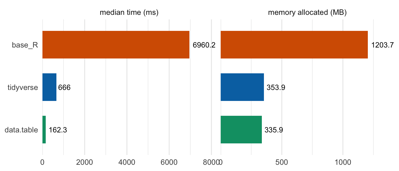
base_R 6.96s 1.18GB
tidyverse 666.01ms 353.88MB
data.table 162.29ms 335.94MB
bench_fig(bench_join, c("base_R", "tidyverse", "data.table"))
Figure 2: Three-table join over 2,000,000 genotype rows: median run time and memory allocated, per engine. Lower is better.

5.3 Reading a file

Large analyses often start by reading a file. Write the genotype table to a temporary TSV, then compare read speeds.

tmp <- tempfile(fileext = ".tsv")
data.table::fwrite(genotypes, tmp, sep = "\t")
cat("file size:", round(file.info(tmp)$size / 1e6, 1), "MB\n")

bench_io <- bench::mark(
  base_R     = read.delim(tmp),
  readr      = readr::read_tsv(tmp, show_col_types = FALSE) |> as.data.frame(),
  data.table = data.table::fread(tmp),
  check = FALSE, iterations = 3, memory = FALSE
)
bench_io[, c("expression", "median")]
unlink(tmp)
file size: 50 MB
expression median
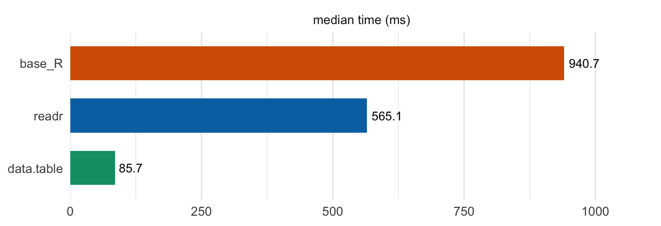
base_R 940.7ms
readr 565.1ms
data.table 85.7ms
bench_fig(bench_io, c("base_R", "readr", "data.table"))
Figure 3: Reading a ~50 MB TSV: median run time, per engine. Lower is better. (Memory is not profiled for file readers, so time only.)

6 Exercises

Each exercise gives the base R and tidyverse answers so you know the target output. Write the data.table version yourself, then open the folded solution to check.

6.1 Per-sample call rate

For each sample, what fraction of genotypes are non-missing (genotype >= 0)? Show the 3 samples with the lowest call rate.

# base R
cr <- sort(tapply(genotypes_df$genotype >= 0, genotypes_df$sample_id, mean))
head(data.frame(sample_id = names(cr), call_rate = as.numeric(cr)), 3)

# tidyverse
genotypes_df |>
  group_by(sample_id) |>
  summarise(call_rate = mean(genotype >= 0)) |>
  arrange(call_rate) |>
  head(3)
sample_id call_rate
S00102 0.97400
S00193 0.97475
S00098 0.97500
sample_id call_rate
S00102 0.97400
S00193 0.97475
S00098 0.97500
Show data.table solution
genotypes[, .(call_rate = mean(genotype >= 0)), by = sample_id][order(call_rate)][1:3]
sample_id call_rate
S00102 0.97400
S00193 0.97475
S00098 0.97500

6.2 High-quality missense rows per gene

Among genotype rows with genotype_quality >= 30 and genotype > 0, joined to variant annotation and keeping consequence == "missense", which 3 genes have the most such rows?

# base R
g  <- genotypes_df[genotypes_df$genotype_quality >= 30 & genotypes_df$genotype > 0, ]
mg <- merge(g, variants_df[, c("variant_id", "consequence", "gene")], by = "variant_id")
tab <- sort(table(mg$gene[mg$consequence == "missense"]), decreasing = TRUE)
head(data.frame(gene = names(tab), n = as.integer(tab)), 3)

# tidyverse
genotypes_df |>
  filter(genotype_quality >= 30, genotype > 0) |>
  inner_join(variants_df, by = "variant_id") |>
  filter(consequence == "missense") |>
  count(gene, sort = TRUE) |>
  head(3)
gene n
GENE0322 812
GENE0714 536
GENE0764 497
gene n
GENE0322 812
GENE0714 536
GENE0764 497
Show data.table solution
variants[genotypes[genotype_quality >= 30 & genotype > 0], on = "variant_id"][
  consequence == "missense", .N, by = gene][order(-N)][1:3]
gene N
GENE0322 812
GENE0714 536
GENE0764 497

6.3 Kept calls per population

Joining genotypes to samples, for each population how many genotype rows pass read_depth >= 15 & genotype_quality >= 25?

# base R
mp   <- merge(genotypes_df, samples_df[, c("sample_id", "population")], by = "sample_id")
keep <- mp$read_depth >= 15 & mp$genotype_quality >= 25
kept <- tapply(keep, mp$population, sum)
data.frame(population = names(kept), kept = as.integer(kept))

# tidyverse
genotypes_df |>
  inner_join(select(samples_df, sample_id, population), by = "sample_id") |>
  group_by(population) |>
  summarise(kept = sum(read_depth >= 15 & genotype_quality >= 25))
population kept
AFR 495340
AMR 291635
EAS 335565
EUR 603131
SAS 271613
population kept
AFR 495340
AMR 291635
EAS 335565
EUR 603131
SAS 271613
Show data.table solution
samples[genotypes, on = "sample_id"][
  , .(kept = sum(read_depth >= 15 & genotype_quality >= 25)), by = population][order(population)]
population kept
AFR 495340
AMR 291635
EAS 335565
EUR 603131
SAS 271613

7 Cheat sheet

Task base R tidyverse data.table
filter rows x[x$a > 1, ] filter(x, a > 1) x[a > 1]
select cols x[, c("a", "b")] select(x, a, b) x[, .(a, b)]
new col x$z <- x$a + x$b mutate(x, z = a + b) x[, z := a + b]
summarise aggregate(a ~ g, x, mean) summarise(x, m = mean(a)) x[, .(m = mean(a))]
group (via aggregate / tapply) group_by(x, g) x[, ..., by = g]
count table(x$g) count(x, g) x[, .N, by = g]
arrange x[order(-x$a), ] arrange(x, desc(a)) x[order(-a)]
join merge(x, y, by = "k") inner_join(x, y, by = "k") x[y, on = "k"], or merge(x, y, by = "k")
read tsv read.delim(f) read_tsv(f) fread(f)
write tsv write.table(x, f) write_tsv(x, f) fwrite(x, f)

8 A caveat: whose method is actually running?

The “base R” column above assumes a plain data.frame. That matters, because data.table inherits from data.frame and supplies its own methods for several base R generics – so identical-looking code can dispatch to a completely different implementation depending on what you hand it. merge() is the clearest example:

dt_x <- data.table(k = 1:3, v = 1:3)
df_x <- as.data.frame(dt_x)

"merge.data.table" %in% as.character(methods("merge"))  # data.table defines one
class(merge(dt_x, dt_x, by = "k"))                      # -> merge.data.table ran
class(merge(df_x, df_x, by = "k"))                      # -> merge.data.frame ran
[1] TRUE
[1] "data.table" "data.frame"
[1] "data.frame"

Hand merge() two data.tables and you get data.table’s own C join, which on millions of rows is more than an order of magnitude faster than base R’s merge.data.frame on the same data – so merge() is a perfectly good data.table join, not just a base R one. The same applies to [: a data.table uses [.data.table, not [.data.frame.

This is exactly why the base R benchmarks above use the _df copies: to measure base R itself, rather than data.table wearing a base R coat. Functions with no data.table method – aggregate(), tapply(), table(), order() – are genuinely base R whatever you pass them.

9 Where to go next

  • vignette("datatable-intro") and the other built-in data.table vignettes
  • ?data.table for the full [i, j, by] reference
  • The dtplyr package: write dplyr code, get data.table speed
  • setDTthreads() / getDTthreads() to tune parallelism

10 Session

Session info
sessionInfo()
R version 4.3.2 (2023-10-31)
Platform: aarch64-apple-darwin20 (64-bit)
Running under: macOS Sonoma 14.8.4

Matrix products: default
BLAS:   /Library/Frameworks/R.framework/Versions/4.3-arm64/Resources/lib/libRblas.0.dylib 
LAPACK: /Library/Frameworks/R.framework/Versions/4.3-arm64/Resources/lib/libRlapack.dylib;  LAPACK version 3.11.0

locale:
[1] C

time zone: Europe/Stockholm
tzcode source: internal

attached base packages:
[1] stats     graphics  grDevices utils     datasets  methods   base     

other attached packages:
[1] ggplot2_3.5.2     bench_1.1.4       readr_2.1.5       dplyr_1.1.4      
[5] data.table_1.17.8

loaded via a namespace (and not attached):
 [1] bit_4.6.0          gtable_0.3.6       jsonlite_2.0.0     crayon_1.5.3      
 [5] compiler_4.3.2     tidyselect_1.2.1   parallel_4.3.2     dichromat_2.0-0.1 
 [9] scales_1.4.0       yaml_2.3.10        fastmap_1.2.0      R6_2.6.1          
[13] labeling_0.4.3     generics_0.1.4     knitr_1.50         htmlwidgets_1.6.4 
[17] tibble_3.3.0       pillar_1.11.1      RColorBrewer_1.1-3 tzdb_0.5.0        
[21] rlang_1.1.6        xfun_0.52          bit64_4.6.0-1      cli_3.6.5         
[25] withr_3.0.2        magrittr_2.0.3     digest_0.6.37      grid_4.3.2        
[29] vroom_1.6.5        hms_1.1.4          lifecycle_1.0.4    vctrs_0.6.5       
[33] evaluate_1.0.5     glue_1.8.0         farver_2.1.2       profmem_0.7.0     
[37] rmarkdown_2.30     tools_4.3.2        pkgconfig_2.0.3    htmltools_0.5.8.1