class: center, middle, inverse, title-slide # Machine Learning in R ## RaukR 2019 • Advanced R for Bioinformatics ### <b>Nikolay Oskolkov</b> ### NBIS, SciLifeLab --- exclude: true count: false <link href="https://fonts.googleapis.com/css?family=Roboto|Source+Sans+Pro:300,400,600|Ubuntu+Mono&amp;subset=latin-ext" rel="stylesheet"> <!-- ----------------- Only edit title & author above this ----------------- --> --- name: Machine Learning for Everyone ## Machine Learning for Everyone .center[ <img src="MachineLearningEveryone.png" style="width: 100%;" />] --- name: Stereotypes about Machine Learning ## Stereotypes about Machine Learning .center[ <img src="MLStereotypes.png" style="width: 90%;" />] --- name: Data Science and Artificial Intelligence ## Data Science and Artificial Intelligence * The world’s most valuable resource is no longer oil, but Data * Big Data is arriving, Bioinformatics learns from Data Science * Data Science speaks Python, Julia, Java Script, Scala and R * Apache Spark, Probabilistic Programming and AI become common .center[ <img src="Oil_vs_Data.jpg" style="width: 90%;" />] --- name: What is Machine Learning? ## What is Machine Learning? * Machine Learning maps input X to output Y as `$$Y = f ( X )$$` without necessarily knowing the functional form of f * Machine Learning provides two major things: * **Prediction** * **Feature Selection** * Machine Learning can be categorized into: * **Parametric**: assumtion on f(X), often linear, easy to learn, fast, little data needed, poor prediction (example: Linear and Logistic Regression) * **Non-Parametric**: assumtion free, difficult to train, slow, needs a lot of data, higher prediction power (example: Random Forest, LASSO, Neural Networks) --- name: Diversity of Machine Learning ## Diversity of Machine Learning 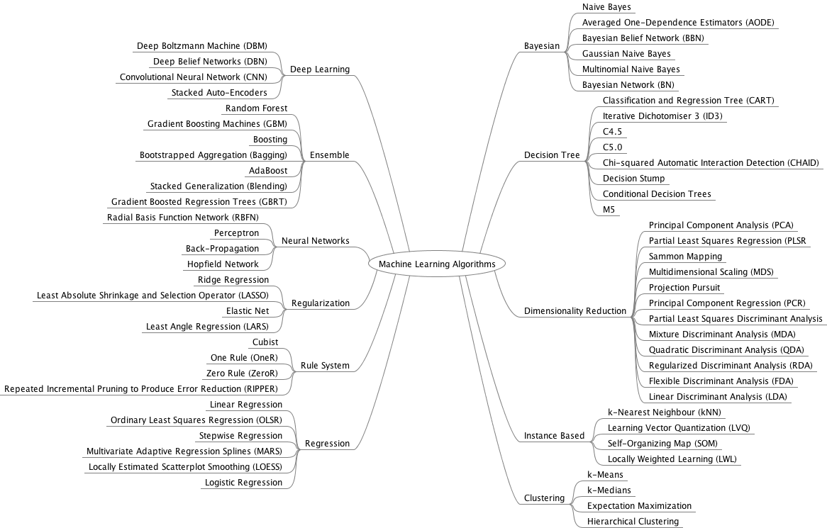 --- name: Supervised vs. Unsupervised ## Supervised vs. Unsupervised .center[ <img src="SupervisedVsUnsupervisedAnalysis.png" style="width: 90%;" />] --- name: Main Steps of Machine Learning ## Main Steps of Machine Learning * To start Machine Learning one needs first to clean the data: impute, correct for batch-effects, normalize, standardize etc. * Next step is to figure out features in the data. Note: Deep Learning skips this step and works directly on raw data * Machine Learning model is fitted on the training and evaluated on an independent subset  --- name: How does Machine Learning work? ## How does Machine Learning work? Machine Learning by default involves five basic steps: 1. Split data set into **train**, **validation** and **test** subsets. 2. Fit the model in the train subset. 3. Validate your model on the validation subset. 4. Repeat steps 1-3 a number of times and tune **hyperparameters**. 5. Test the accuracy of the optimized model on the test subset. .center[ <img src="TrainTestSplit.png" style="width: 60%;" />] --- name: Toy Example of Machine Learning ## Toy Example of Machine Learning ```r set.seed(12345) N<-100 x<-rnorm(N) y<-2*x+rnorm(N) df<-data.frame(x,y) plot(y~x,data=df, col="blue") ``` <img src="Presentation_MachineLearning_files/figure-html/unnamed-chunk-3-1.svg" style="display: block; margin: auto;" /> --- name: Train and Test Subsets ## Train and Test Subsets We randomly assign 70% of the data to training and 30% to test subsets: ```r set.seed(123) train<-df[sample(1:dim(df)[1],0.7*dim(df)[1]),] test<-df[!rownames(df)%in%rownames(train),] ``` <img src="Presentation_MachineLearning_files/figure-html/unnamed-chunk-5-1.svg" style="display: block; margin: auto;" /> --- name: Validation of Model ## Validation of Model ```r test_predicted<-as.numeric(predict(lm(y~x,data=train),newdata=test)) plot(test$y~test_predicted,ylab="True y",xlab="Pred y",col="darkgreen") abline(lm(test$y~test_predicted),col="darkgreen") ``` <img src="Presentation_MachineLearning_files/figure-html/unnamed-chunk-6-1.svg" style="display: block; margin: auto;" /> --- name: Validation of Model (Cont.) ## Validation of Model (Cont.) ```r summary(lm(test$y~test_predicted)) ``` ``` ## ## Call: ## lm(formula = test$y ~ test_predicted) ## ## Residuals: ## Min 1Q Median 3Q Max ## -1.80597 -0.78005 0.07636 0.52330 2.61924 ## ## Coefficients: ## Estimate Std. Error t value Pr(>|t|) ## (Intercept) 0.02058 0.21588 0.095 0.925 ## test_predicted 0.89953 0.08678 10.366 4.33e-11 *** ## --- ## Signif. codes: 0 '***' 0.001 '**' 0.01 '*' 0.05 '.' 0.1 ' ' 1 ## ## Residual standard error: 1.053 on 28 degrees of freedom ## Multiple R-squared: 0.7933, Adjusted R-squared: 0.7859 ## F-statistic: 107.4 on 1 and 28 DF, p-value: 4.329e-11 ``` Thus the model explains 79% of variation on the test subset. --- name: What is a Hyperparameter? ## What is a Hyperparameter? * Hyperparameters are Machine Learning design parameters which are set before the learning process starts * For the toy model a hyperparameter can be e.g. the number of covariates to adjust the main variable x of interest for ```r set.seed(1) for(i in 1:10) { df[,paste0("PC",i)]<-1*(1-i/10)*y+rnorm(N) } head(df) ``` ``` ## x y color PC1 PC2 PC3 PC4 ## 1 0.5855288 1.3949830 red 0.6290309 0.4956198 1.3858900 1.7306635 ## 2 0.7094660 0.2627087 red 0.4200812 0.2522828 1.8727694 -0.8896729 ## 3 -0.1093033 0.2038119 red -0.6521979 -0.7478721 1.7292568 2.0936245 ## 4 -0.4534972 -2.2317496 blue -0.4132938 -1.6273709 -1.8931325 -1.7226819 ## 5 0.6058875 1.3528592 blue 1.5470811 0.4277027 -1.3382341 2.4658608 ## 6 -1.8179560 -4.1719599 blue -4.5752323 -1.5702807 -0.4227104 -0.9909633 ## PC5 PC6 PC7 PC8 PC9 PC10 ## 1 1.7719325 0.63529634 0.07742793 -0.4285716 -0.9474105 -1.5414026 ## 2 2.0270091 -0.19178516 1.58123715 2.0241138 -1.7998121 0.1943211 ## 3 -0.5010914 -1.10171748 0.58945128 -0.0492363 1.0156630 0.2644225 ## 4 -1.5067426 -0.88140715 -0.12733353 -0.4603672 -0.2350367 -1.1187352 ## 5 0.2602076 1.53274473 0.26918441 -0.8528851 -0.4643425 0.6509530 ## 6 -2.4616374 -0.07481652 -2.38832183 -2.1785221 -0.5951440 -1.0329002 ``` --- name: How does Cross-Validation work? ## How does Cross-Validation work? * We should not include all PCs - overfitting * Cross-Validation is a way to combat overfitting ```r train<-df[sample(1:dim(df)[1],0.6*dim(df)[1]),] val_test<-df[!rownames(df)%in%rownames(train),] validate<-val_test[sample(1:dim(val_test)[1],0.25*dim(val_test)[1]),] test<-val_test[!rownames(val_test)%in%rownames(validate),] ``` <img src="Presentation_MachineLearning_files/figure-html/unnamed-chunk-10-1.svg" style="display: block; margin: auto;" /> --- name: How does Cross-Validation work? (Cont.) ## How does Cross-Validation work? (Cont.) * Let us fit the linear regression model in the training set and validate the error in the validation data set * Error: root mean squared difference between y predicted by the trained model for validation set and the real y in the validation set * Looks like no drammatic decrease of RMSE after PC2 <img src="Presentation_MachineLearning_files/figure-html/unnamed-chunk-11-1.svg" style="display: block; margin: auto;" /> --- name: Ultimate Model Evaluation ## Ultimate Model Evaluation * Thus optimal model is y~x+PC1+PC2 * Perform final evaluation of the optimized/trained model on the test data set and report the final accuracy (adjusted R squared) * The model explains over 90% of variation on the unseen test data set ```r summary(lm(predict(lm(y~x+PC1+PC2,data=train),newdata=test)~test$y)) ``` ``` ## ## Call: ## lm(formula = predict(lm(y ~ x + PC1 + PC2, data = train), newdata = test) ~ ## test$y) ## ## Residuals: ## Min 1Q Median 3Q Max ## -1.02409 -0.26361 -0.00061 0.19345 0.95801 ## ## Coefficients: ## Estimate Std. Error t value Pr(>|t|) ## (Intercept) 0.22155 0.09485 2.336 0.0269 * ## test$y 0.93912 0.03994 23.514 <2e-16 *** ## --- ## Signif. codes: 0 '***' 0.001 '**' 0.01 '*' 0.05 '.' 0.1 ' ' 1 ## ## Residual standard error: 0.5002 on 28 degrees of freedom ## Multiple R-squared: 0.9518, Adjusted R-squared: 0.9501 ## F-statistic: 552.9 on 1 and 28 DF, p-value: < 2.2e-16 ``` --- name: Underfitting vs. Overfitting ## Underfitting vs. Overfitting 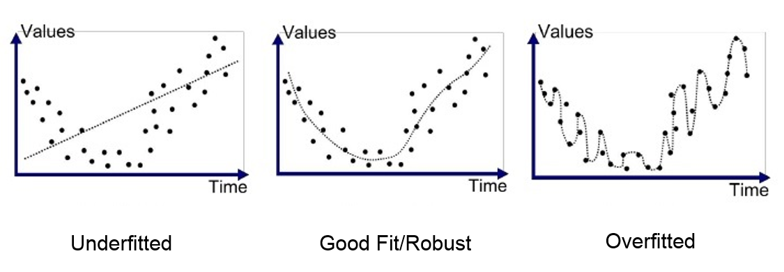 * Akaike Information Criterion (AIC): `$$\rm AIC = 2k - 2ln(L)$$` * Random Forest: each tree overfitted, but ensemble of trees performs very well --- name: Bias-Variance ## Bias-Variance Tradeoff .pull-left-50[ 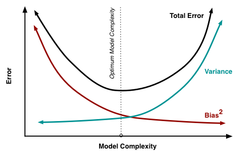 ] .pull-right-50[ 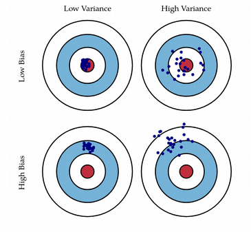 ] `$$Y = f(X) \Longrightarrow\rm{Reality} \\ Y = \hat{f}(X) + \rm{Error}\Longrightarrow\rm{Model} \\ Error^2 = (Y - \hat{f}(X))^2 = Bias^2 + Variance$$` * It is mathematically proven that ensemble learning keeps the Bias the same but leads to a large decrease of Variance --- name: KNN and SVM ## KNN and SVM .pull-left-50[  * How many out of K neighbors belong to each class * Majority voting * Non-linear ] .pull-right-50[  * Draw hyperplane that separates classes * Maximize margins * Can be linear and non-linear ] --- name: Random Forest ## What is Random Forest?  --- name: Classification: Pima Indians Diabetes ## Classification: Pima Indians Diabetes ```r library("mlbench") data(PimaIndiansDiabetes2) head(PimaIndiansDiabetes2,4) ``` ``` ## pregnant glucose pressure triceps insulin mass pedigree age diabetes ## 1 6 148 72 35 NA 33.6 0.627 50 pos ## 2 1 85 66 29 NA 26.6 0.351 31 neg ## 3 8 183 64 NA NA 23.3 0.672 32 pos ## 4 1 89 66 23 94 28.1 0.167 21 neg ``` ```r summary(results) ``` ``` ## ## Call: ## summary.resamples(object = results) ## ## Models: lda, cart, knn, svm, rf ## Number of resamples: 50 ## ## ROC ## Min. 1st Qu. Median Mean 3rd Qu. Max. NA's ## lda 0.6240602 0.8075188 0.8496241 0.8387103 0.8780739 0.9488722 0 ## cart 0.5766917 0.6664197 0.7097966 0.7213344 0.7794339 0.9195046 0 ## knn 0.6408669 0.7710305 0.8120301 0.8108961 0.8377820 0.9699248 0 ## svm 0.7293233 0.8034056 0.8337240 0.8349049 0.8735294 0.9609023 0 ## rf 0.7187970 0.7934211 0.8417293 0.8316356 0.8721805 0.9195489 0 ## ## Sens ## Min. 1st Qu. Median Mean 3rd Qu. Max. NA's ## lda 0.7352941 0.8285714 0.8857143 0.8758655 0.9142857 1.0000000 0 ## cart 0.5588235 0.7771008 0.8285714 0.8296303 0.8857143 0.9714286 0 ## knn 0.6285714 0.7941176 0.8260504 0.8188571 0.8571429 1.0000000 0 ## svm 0.7428571 0.8285714 0.8571429 0.8634958 0.8857143 1.0000000 0 ## rf 0.7142857 0.8000000 0.8285714 0.8417143 0.8857143 1.0000000 0 ## ## Spec ## Min. 1st Qu. Median Mean 3rd Qu. Max. NA's ## lda 0.3157895 0.4868421 0.5789474 0.5652632 0.6315789 0.7894737 0 ## cart 0.3157895 0.4736842 0.5263158 0.5547368 0.6710526 0.7894737 0 ## knn 0.4210526 0.5789474 0.6315789 0.6252632 0.7236842 0.8421053 0 ## svm 0.3684211 0.4736842 0.5789474 0.5631579 0.6315789 0.7894737 0 ## rf 0.3684211 0.5263158 0.6315789 0.6136842 0.7236842 0.7894737 0 ``` --- name: Compare Machine Learning Methods ## Compare Machine Learning Methods ```r dotplot(results) ``` <img src="Presentation_MachineLearning_files/figure-html/unnamed-chunk-16-1.svg" style="display: block; margin: auto auto auto 0;" /> --- name: Feature Selection ## Feature Selection ```r feat<-varImp(best_model)$importance$pos names(feat)<-rownames(varImp(best_model)$importance) barplot(sort(feat,decreasing=T),ylab="FEATURE IMPORTANCE",col="darkred") ``` <img src="Presentation_MachineLearning_files/figure-html/unnamed-chunk-18-1.svg" style="display: block; margin: auto auto auto 0;" /> --- name: Make Predictions ## Make Predictions: Confusion Matrix ```r library("e1071") predictions <- predict(best_model, test) confusionMatrix(predictions, test$diabetes) ``` ``` ## Confusion Matrix and Statistics ## ## Reference ## Prediction neg pos ## neg 132 32 ## pos 21 46 ## ## Accuracy : 0.7706 ## 95% CI : (0.7109, 0.8232) ## No Information Rate : 0.6623 ## P-Value [Acc > NIR] : 0.0002237 ## ## Kappa : 0.4687 ## ## Mcnemar's Test P-Value : 0.1695641 ## ## Sensitivity : 0.8627 ## Specificity : 0.5897 ## Pos Pred Value : 0.8049 ## Neg Pred Value : 0.6866 ## Prevalence : 0.6623 ## Detection Rate : 0.5714 ## Detection Prevalence : 0.7100 ## Balanced Accuracy : 0.7262 ## ## 'Positive' Class : neg ## ``` --- name: ROC Curves ## ROC Curves on Test Data Set <img src="Presentation_MachineLearning_files/figure-html/unnamed-chunk-20-1.svg" style="display: block; margin: auto;" /> --- name: Why such a hype about Deep Learning? ## Why such a hype about Deep Learning? .center[ <img src="DLHype.png" style="width: 100%;" />] .center[ <span style="color:red">**Because Deep Learning delivers state-of-the-art results**</span>] --- name: Promises of Deep Learning for Society ## Promises of Deep Learning for Society .center[ <img src="DLPromises.png" style="width: 90%;" />] --- name: Promises of Deep Learning for Life Sciences ## Promises of Deep Learning for Life Sciences .center[ <img src="DLLifeSciences.png" style="width: 80%;" />] --- name: What is Deep Learning? ## What is Deep Learning? * Artificial Neural Networks (ANN) with multiple layers * Main advantages of Deep Learning over Machine Learning: * Feature extraction * Scalability * Universal Approximation Theorem <img src="Presentation_MachineLearning_files/figure-html/unnamed-chunk-21-1.svg" style="display: block; margin: auto;" /> --- name: Artificial Neural Networks (ANN) ## Artificial Neural Networks (ANN) * Mathematical algorithm/function with special architecture * Highly non-linear dues to activation functions * Backward propagation for minimizing error .center[ <img src="ANN.png" style="width: 90%;" />] --- name: Convolutional Neural Networks (CNN) ## Convolutional Neural Networks (CNN) .center[ <img src="CNN.png" style="width: 100%;" />] --- name: Computer Vision ## Computer Vision .center[ <img src="NASnet.jpg" style="width: 100%;" />] --- name: Object Detection ## Object Detection .pull-left-50[ <img src="RPN.jpeg" style="width: 70%;" />] .pull-right-50[ <img src="SelectiveSearch.png" style="width: 80%;" /> <img src="Faster-rcnn.png" style="width: 80%;" /> ] --- name: Human Protein Atlas ## Human Protein Atlas .center[ <img src="RBC_WBC.png" style="width: 70%;" />] .center[ <img src="HPA.png" style="width: 70%;" />] --- name: Image Annotation ## Image Annotation .center[ <img src="LabelImg.png" style="width: 50%;" />] .center[ <img src="tSNE_cells.png" style="width: 40%;" />] --- name: Beauty of Neural Networks ## Beauty of Neural Networks * Maximum Likelihood * Cross-Validation * Bootstrapping * Regularization * Bayesian Inference * Multivariate Feature Selection * Monte Carlo Approximation * Bagging and Boosting  --- name: Single Cells make Big Data ## Single Cells make Big Data .center[ <img src="SingleCellBigData.png" style="width: 90%;" />] --- name: Autoencoders ## Autoencoders .center[ <img src="Autoencoder.png" style="width: 90%;" />] --- name: Autoencoders for scRNAseq ## Autoencoders for scRNAseq .center[ <img src="AutoencoderscRNAseq.png" style="width: 90%;" />] --- name: Autoencoders for Large-Scale scRNAseq ## Autoencoders for Large-Scale scRNAseq .center[ <img src="Autoencoder10X.png" style="width: 90%;" />] --- name: Frequentist Image Recognition ## Frequentist Image Recognition .center[ <img src="FreqImgRecogn.png" style="width: 90%;" />] --- name: Bayesian Image Recognition ## Bayesian Image Recognition .center[ <img src="BayesImgRecogn.png" style="width: 90%;" />] --- name: Bayesian Deep Learning for Single Cell ## Bayesian Deep Learning for Single Cell .center[ <img src="BayesianDeepLearning.png" style="width: 90%;" />] --- name: Reinforcement Learning ## Reinforcement Learning .center[ <img src="EA_RL.gif.png" style="width: 100%;" />] --- name: Towards Self-Trainable Machines ## Towards Self-Trainable Machines .pull-left-50[ .center[ <img src="ReinforcementLearning.png" style="width: 100%;" /> <img src="QLearning.jpeg" style="width: 100%;" />] ] .pull-right-50[ .center[ <img src="RL_Loss.png" style="width: 100%;" /> <img src="OpenAIGym.jpeg" style="width: 100%;" /> ]] --- name: Bioinformatics Learns from Google ## Bioinformatics Learns from Google .center[ <img src="DeepMind.png" style="width: 90%;" />] --- name: Total Science: Pan-Science ## Total Science: Pan-Science .pull-left-50[ .center[ Total Football <img src="TotalFootball.jpg" style="width: 100%;" />]] .pull-right-50[ .center[ Total Hockey <img src="RedArmy.jpg" style="width: 80%;" />]] .center[ <img src="Leonardo.png" style="width: 60%;" />] <!-- --------------------- Do not edit this and below --------------------- --> --- name: end-slide class: end-slide, middle count: false # Thank you. Questions? <p>R version 3.6.0 (2019-04-26)<br><p>Platform: x86_64-pc-linux-gnu (64-bit)</p><p>OS: Ubuntu 14.04.6 LTS</p><br> Built on : <i class='fa fa-calendar' aria-hidden='true'></i> 16-jun-2019 at <i class='fa fa-clock-o' aria-hidden='true'></i> 17:03:52 __2019__ • [SciLifeLab](https://www.scilifelab.se/) • [NBIS](https://nbis.se/)