Building a Shiny web application to visualize spatial and spatio-temporal data
Paula Moraga
CHICAS, Lancaster University, UK
31 May 2018
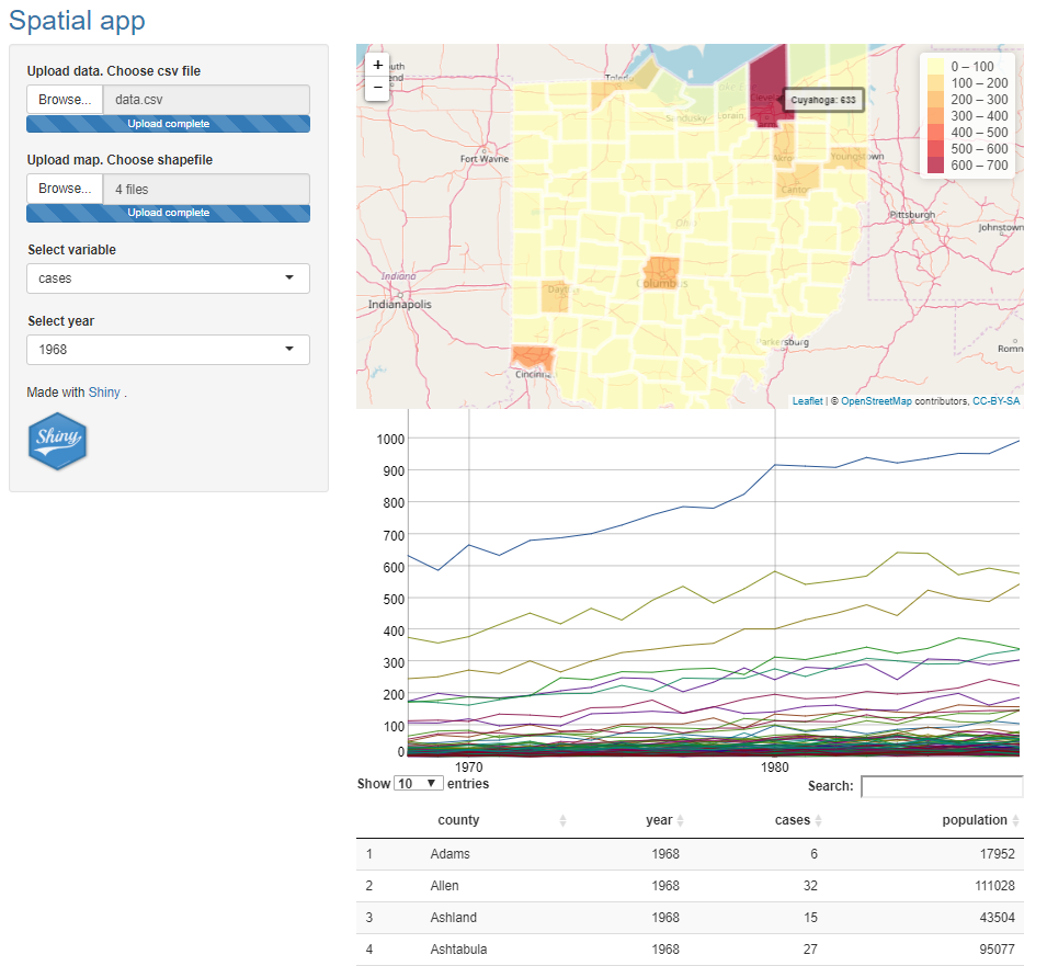
In this tutorial we develop a Shiny web application to visualize spatial and spatio-temporal data. Specifically, the app shows the number of disease cases and the population in a given region using interactive maps, tables, and time series plots. The app allows the user to upload a csv file with the data and a shapefile with the map of the region. The app also permits selecting the variable and the time to be shown.
We develop the app using the R package Shiny. The interactive data visualizations are built using the packages DT, dygraphs, and leaflet. The example we use refers to data of the number of lung cancer cases and population in the 88 counties of Ohio, United States, during years 1968 to 1988. These data are in the package SpatialEpiApp and can also be downloaded from here.
1 Shiny
Shiny is a web application framework for R that enables to build interactive web applications. A Shiny app is a directory that contains an R file called app.R with three components:
- a user interface object (
ui) which controls the layout and appearance of the app, - a
server()function with the instructions to build the objects displayed in theui, - a call to
shinyApp()that creates the Shiny app from theui/serverpair.
Shiny apps contain input and output objects. Inputs permit users interact with the app by modifying their values. Outputs are objects that are shown in the app. Outputs are reactive if they are built using input values.
The content of app.R is as follows.
# load the shiny package
library(shiny)

# define user interface object
ui <- fluidPage(
  *Input(inputId = myinput, label = mylabel, ...)
  *Output(outputId = myoutput, ...)
)

# define server() function
server <- function(input, output){
  output$myoutput <- render*({
    # code to build the output.
    # If it uses an input value (input$myinput),
    # the output will be rebuilt whenever
    # the input value changes
  })}

# call to shinyApp() which returns the Shiny app
shinyApp(ui = ui, server = server)
The app.R file is saved inside a directory called appdir. Then, the app can be launched by typing runApp("appdir_path") where appdir_path is the path of the directory that contains app.R.
2 Setup
We download the folder appdir from here and save it in our computer. This folder contains the following subfolders:
datawhich contains a file calleddata.csvwith the data, and a folder calledfe_2007_39_countywith the shapefile of Ohio,wwwwith the imageimageShiny.png.
3 Structure of app.R
We start by writing a file called app.R with the minimum code needed to create a Shiny app.
library(shiny)

# ui object
ui <- fluidPage( )

# server()
server <- function(input, output){ }

# shinyApp()
shinyApp(ui = ui, server = server)
We save this file with name app.R inside the directory called appdir. Then, we can launch the app by typing clicking the Run App button at the top of the RStudio editor, or by executing runApp("appdir_path") where appdir_path is the path of the directory that contains app.R.
The resulting app has a blank user interface. In the following sections we include the objects and functionality we want to have in the app.
4 Layout
We build a user interface with a sidebar layout. This layout includes a title panel, a sidebar panel for inputs on the left and a main panel for outputs on the right. The elements of the user interface are placed within the fluidPage() function and this permits the app to be automatically adjust to the dimensions of the browser window.
The title of the app is added with titlePanel(). Then we write sidebarLayout() to create a sidebar layout with input and output definitions. sidebarLayout() takes the arguments sidebarPanel() and mainPanel(). sidebarPanel() creates a a sidebar panel for inputs on the left. mainPanel() creates a main panel for displaying outputs on the right.
ui <- fluidPage(
  titlePanel("title"),
  sidebarLayout(
    sidebarPanel("sidebar panel for inputs"),
    mainPanel("main panel for outputs")
  )
)
We can add content to the app by passing it as an argument to titlePanel(), sidebarPanel(), or mainPanel(). Here we have added texts with the description of the panels.
Note that to include multiple elements in the same panel they need to be separated with a comma.
5 HTML content
Now we add content to the app.
5.1 Add title
First we add the title “Spatial app” to titlePanel(). We want to show this title in blue so we use p() to create a paragraph with text and set the style to #3474A7 color.
titlePanel(p("Spatial app", style = "color:#3474A7")),5.2 Add image
Now we add an image with the img() function. The images that we wish to include in the app must be in a folder named www in the same directory as the app.R file. We use an image called imageShiny.png and put it in the sidebarPanel() using the following instruction.
sidebarPanel(img(src = "imageShiny.png", width = "70px", height = "70px")),Here src denotes the source of the image, and height and width are the image height and width in pixels, respectively.
5.3 Add website link
We also add a text with a link referencing the Shiny website.
p("Made with", a("Shiny", href = "http://shiny.rstudio.com"), "."),Note that in sidebarPanel() we need to write the function to generate the website link and the function to include the image separated with a comma.
sidebarPanel(
p("Made with", a("Shiny", href = "http://shiny.rstudio.com"), "."),
img(src = "imageShiny.png", width = "70px", height = "70px")),
6 Content of app.R
This is the content of app.R we have until now.
library(shiny)

# ui object
ui <- fluidPage(
  titlePanel(p("Spatial app", style = "color:#3474A7")),
  sidebarLayout(
    sidebarPanel(
      p("Made with", a("Shiny", href = "http://shiny.rstudio.com"), "."),
      img(src = "imageShiny.png", width = "70px", height = "70px")),
    mainPanel("main panel for outputs")
  )
)

# server()
server <- function(input, output){ }

# shinyApp()
shinyApp(ui = ui, server = server)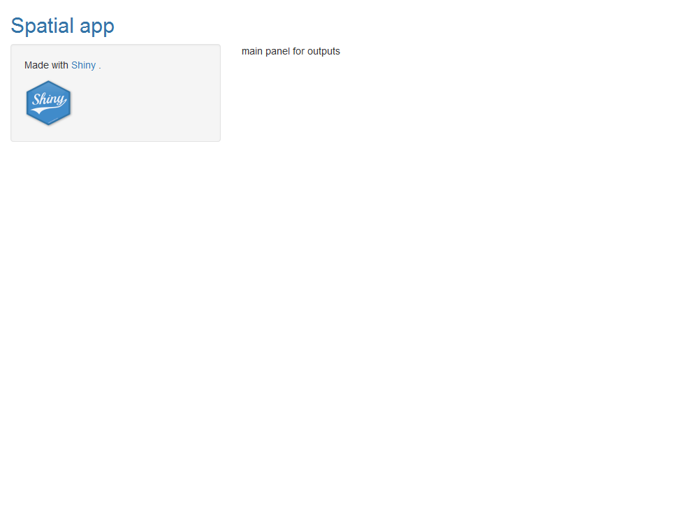
7 Read data
Now we read the data we want to show in the app. The data is in the folder called data in the appdir directory. We load the rgdal package, read the data data.csv, and read the shapefile of Ohio which is in the folder fe_2007_39_county.
library(rgdal)
data <- read.csv("data/data.csv")
map <- readOGR("data/fe_2007_39_county/fe_2007_39_county.shp")
We only need to read the data once so we write this code at the beginning of app.R outside the server() function. By doing this, the code is not unnecessarily run more than once and the performance of the app is not decreased.
8 Add outputs
The server() function has the arguments input and output. input is a list-like object that stores the current values of the objects in the app. output is a list-like object that stores instructions for building the R objects in the app. Each element of output contains the output of a render*() function.
We show the data using several outputs. Outputs are added in the app by including in ui an *Output() function for the output, and adding in server() a render*() function to the output that specifies how to build the object. For example, to add a plot, we write in the ui plotOutput() and in server() renderPlot().
Here we include three outputs for interactive visualization. These are HTML widgets created with JavaScript libraries and embedded in Shiny by using the htmlwidgets package. The outputs are created using the following packages:
DTto display the data in an interactive table,dygraphsto display time series data,leafletto create an interactive map.
8.1 Table using DT
https://rstudio.github.io/DT/shiny.html
We show the data stored in data with an interactive table using the DT package. In ui we use DTOutput(), and in server() we use renderDT().
library(DT)

# in ui
DTOutput(outputId = "table")

# in server()
output$table <- renderDT(data)
8.2 Time series plot using dygraphs
http://rstudio.github.io/dygraphs
We show the temporal trends of the data with the dygraphs package. In ui we use dygraphOutput(), and in server() we use renderDygraph().
dygraphs plots an extensible time series object xts. We can create this type of object using the xts() function of the xts package specifying the values and the dates. The dates in data are the years of column year. For now we choose to plot the values of the variable cases of data.
We need to construct a xts for each county and then put them together in dataxts. For each of the counties, we filter the data of the county and assign it to datacounty. Then we construct a xts object with values datacounty$cases and dates as.Date(paste0(data$year, "-01-01")). Then we assign the name of the counties to each xts (colnames(dataxts) <- counties) so county names can be shown in the legend.
dataxts <- NULL
counties <- unique(data$county)
for(l in 1:length(counties)){
  datacounty <- data[data$county == counties[l],]
  dd <- xts(datacounty[, "cases"], as.Date(paste0(datacounty$year, "-01-01")))
  dataxts <- cbind(dataxts, dd)
}
colnames(dataxts) <- counties
Finally we plot dataxts with dygraph() allowing for mouse-over highlighting.
dygraph(dataxts) %>% dyHighlight(highlightSeriesBackgroundAlpha = 0.2)We customize the legend so only the name of the highlighted serie is shown. To do this, one option is writing a css file with the instructions and pass the css file to dyCSS(). Instead of that, we set the css directly in the code as shown here.
dygraph(dataxts) %>% dyHighlight(highlightSeriesBackgroundAlpha = 0.2) -> d1

d1$x$css = "
.dygraph-legend > span {display:none;}
.dygraph-legend > span.highlight { display: inline; }
"
d1
The complete code to build the dygraphs object is the following:
library(dygraphs)
library(xts)

# in ui
dygraphOutput(outputId = "timetrend")

# in server()
output$timetrend <- renderDygraph({

  dataxts <- NULL
  counties <- unique(data$county)
  for(l in 1:length(counties)){
    datacounty <- data[data$county == counties[l], ]
    dd <- xts(datacounty[, "cases"], as.Date(paste0(datacounty$year, "-01-01")))
    dataxts <- cbind(dataxts, dd)
  }
  colnames(dataxts) <- counties

  dygraph(dataxts) %>% dyHighlight(highlightSeriesBackgroundAlpha = 0.2)-> d1

  d1$x$css = "
 .dygraph-legend > span {display:none;}
 .dygraph-legend > span.highlight { display: inline; }
 "
  d1
})
8.3 Map using leaflet
http://rstudio.github.io/leaflet/
We use the leaflet package to build an interactive map. In ui we use leafletOutput(), and in server() we use renderLeaflet(). Inside renderLeaflet() we write the instructions to return a leaflet map.
First, we need to add the data to the shapefile so the values can be plotted in a map. For now we choose to plot the values of the variable in year 1980. We create a dataset datafiltered with the data corresponding to that year. Then we add datafiltered to map@data in an order such that the counties in the data match the counties in the map.
datafiltered <- data[which(data$year == 1980), ]
# this returns positions of `map@data$NAME` in `datafiltered$county`
ordercounties <- match(map@data$NAME, datafiltered$county)
map@data <- datafiltered[ordercounties, ]
We create the leaflet map following the instructions here. We use the leaflet() function, create a colour palette with colorBin(), and add a legend with addLegend(). For now we choose to plot the values of variable cases. We also add labels with the area names and values that are displayed when mouse is over the map.
library(leaflet)

# in ui
leafletOutput(outputId = "map")

# in server()
output$map <- renderLeaflet({

  # Add data to map
  datafiltered <- data[which(data$year == 1980), ]
  ordercounties <- match(map@data$NAME, datafiltered$county)
  map@data <- datafiltered[ordercounties, ]

  # Create leaflet
  pal <- colorBin("YlOrRd", domain = map$cases, bins = 7)

  labels <- sprintf("%s: %g", map$county, map$cases) %>% lapply(htmltools::HTML)

  l <- leaflet(map) %>% addTiles() %>% addPolygons(
    fillColor = ~pal(cases),
    color = "white",
    dashArray = "3",
    fillOpacity = 0.7,
    label = labels) %>%
    leaflet::addLegend(pal = pal, values = ~cases, opacity = 0.7, title = NULL)
})
9 Content of app.R
This is the content of app.R we have until now.
library(shiny)
library(rgdal)
library(DT)
library(dygraphs)
library(xts)
library(leaflet)

data <- read.csv("data/data.csv")
map <- readOGR("data/fe_2007_39_county/fe_2007_39_county.shp")

# ui object
ui <- fluidPage(
  titlePanel(p("Spatial app", style = "color:#3474A7")),
  sidebarLayout(
    sidebarPanel(
      p("Made with", a("Shiny", href = "http://shiny.rstudio.com"), "."),
      img(src = "imageShiny.png", width = "70px", height = "70px")),
    mainPanel(
      leafletOutput(outputId = "map"),
      dygraphOutput(outputId = "timetrend"),
      DTOutput(outputId = "table")
    )
  )
)

# server()
server <- function(input, output){
  output$table <- renderDT(data)

  output$timetrend <- renderDygraph({

    dataxts <- NULL
    counties <- unique(data$county)
    for(l in 1:length(counties)){
      datacounty <- data[data$county == counties[l],]
      dd <- xts(datacounty[, "cases"], as.Date(paste0(datacounty$year,"-01-01")))
      dataxts <- cbind(dataxts, dd)
    }
    colnames(dataxts) <- counties

    dygraph(dataxts) %>% dyHighlight(highlightSeriesBackgroundAlpha = 0.2)-> d1

    d1$x$css = "
 .dygraph-legend > span {display:none;}
 .dygraph-legend > span.highlight { display: inline; }
 "
    d1
  })

  output$map <- renderLeaflet({

    # Add data to map
    datafiltered <- data[which(data$year == 1980), ]
    ordercounties <- match(map@data$NAME, datafiltered$county)
    map@data <- datafiltered[ordercounties, ]

    # Create leaflet
    pal <- colorBin("YlOrRd", domain = map$cases, bins = 7)

    labels <- sprintf("%s: %g", map$county, map$cases) %>% lapply(htmltools::HTML)

    l <- leaflet(map) %>% addTiles() %>% addPolygons(
      fillColor = ~pal(cases),
      color = "white",
      dashArray = "3",
      fillOpacity = 0.7,
      label = labels) %>%
      leaflet::addLegend(pal = pal, values = ~cases, opacity = 0.7, title = NULL)
    # write leaflet::addLegend to avoid Error object '.xts_chob' not found
  })
}

# shinyApp()
shinyApp(ui = ui, server = server)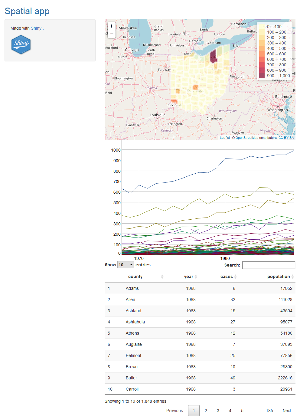
10 Add reactivity
Now we add functionality to enable users select a specific variable and year to be shown. In order to select a variable, we include an input of a menu containing the possible variables. Then the user can select the variable he or she wants to see, and this will rebuild the map and the time series plot.
To add an input to a Shiny app, we need to place an input function *Input() in the ui object. Each input function requires several arguments. The first two are inputId, a name necessary to access the input’s value, and label, a label that appears in the app. We create the input menu with the possible variable choices using this code.
# in ui
selectInput(inputId = "variableselected"", label = "Select variable",
            choices = c("cases", "population"))
In this input, name is "variableselected", label is "Select variable" and choices contains the variables to select from which are "cases" and "population". The value of this input can be accessed with input$variableselected. We create reactivity by including the value of the input (input$variableselected) in the render*() expressions in server() that build the outputs. Thus, when we select a different variable in the menu, Shiny rebuilds all the outputs that depend on the input using the updated input value.
Similarly, we add a menu with name "yearselected" with all possible years so we can select the year we want to see. The name of this input is "yearselected". When we select a year, the input value input$yearselected changes and Shiny rebuilds all the outputs that depend on it using the new input value.
# in ui
selectInput(inputId = "yearselected", label = "Select year",
            choices = 1968:1988)
Now we need to modify the dygraphs time series plot and the leaflet map so that they are built with the input values input$variableselected and input$yearselected.
10.1 Reactivity in dygraphs
We modify renderDygraph() by writing datacounty[, input$variableselected] instead of datacounty$cases.
# in server()
output$timetrend <- renderDygraph({

  dataxts <- NULL
  counties <- unique(data$county)
  for(l in 1:length(counties)){
    datacounty <- data[data$county == counties[l], ]
    dd <- xts(datacounty[, input$variableselected], as.Date(paste0(datacounty$year, "-01-01"))) # CHANGE "cases" by input$variableselected
    dataxts <- cbind(dataxts, dd)
  }
...
})
10.2 Reactivity in leaflet
We also modify renderLeaflet() by selecting data corresponding to year input$yearselected and plot variable input$variableselected instead of variable cases. We create a new column in map called variableplot with the values of variable input$variableselected and plot the map with the values in variableplot. In leaflet() we modify colorBin(), addPolygons(), addLegend() and labels to show variableplot instead of variable cases.
output$map <- renderLeaflet({

  # Add data to map
  datafiltered <- data[which(data$year == input$yearselected), ] # CHANGE 1980 by input$yearselected
  ordercounties <- match(map@data$NAME, datafiltered$county)
  map@data <- datafiltered[ordercounties, ]

  # Create variableplot
  map$variableplot <- as.numeric(map@data[, input$variableselected]) # ADD this to create variableplot

  # Create leaflet
  pal <- colorBin("YlOrRd", domain = map$variableplot, bins = 7) # CHANGE map$cases by map$variableplot

  labels <- sprintf("%s: %g", map$county, map$variableplot) %>% lapply(htmltools::HTML) # CHANGE map$cases by map$variableplot

  l <- leaflet(map) %>% addTiles() %>% addPolygons(
    fillColor = ~pal(variableplot), # CHANGE cases by variableplot
    color = "white",
    dashArray = "3",
    fillOpacity = 0.7,
    label = labels) %>%
    leaflet::addLegend(pal = pal, values = ~variableplot, opacity = 0.7, title = NULL) # CHANGE cases by variableplot
})
Note that a better way to modify an existing leaflet map is using the leafletProxy() function. Details on how to use this function are given here.
11 Content of app.R
The content of app.R is shown below.
library(shiny)
library(rgdal)
library(DT)
library(dygraphs)
library(xts)
library(leaflet)

data <- read.csv("data/data.csv")
map <- readOGR("data/fe_2007_39_county/fe_2007_39_county.shp")

# ui object
ui <- fluidPage(
  titlePanel(p("Spatial app", style = "color:#3474A7")),
  sidebarLayout(
    sidebarPanel(
      selectInput(inputId = "variableselected", label = "Select variable",
                  choices = c("cases", "population")),
      selectInput(inputId = "yearselected", label = "Select year",
                  choices = 1968:1988),

      p("Made with", a("Shiny", href = "http://shiny.rstudio.com"), "."),
      img(src = "imageShiny.png", width = "70px", height = "70px")
    ),

    mainPanel(
      leafletOutput(outputId = "map"),
      dygraphOutput(outputId = "timetrend"),
      DTOutput(outputId = "table")
    )
  )
)

# server()
server <- function(input, output){
  output$table <- renderDT(data)

  output$timetrend <- renderDygraph({

    dataxts <- NULL
    counties <- unique(data$county)
    for(l in 1:length(counties)){
      datacounty <- data[data$county == counties[l],]
      dd <- xts(datacounty[, input$variableselected], as.Date(paste0(datacounty$year,"-01-01")))
      dataxts <- cbind(dataxts, dd)
    }
    colnames(dataxts) <- counties

    dygraph(dataxts) %>% dyHighlight(highlightSeriesBackgroundAlpha = 0.2)-> d1

    d1$x$css = "
 .dygraph-legend > span {display:none;}
 .dygraph-legend > span.highlight { display: inline; }
 "
    d1
  })

  output$map <- renderLeaflet({

    # Add data to map
    datafiltered <- data[which(data$year == input$yearselected), ] # CHANGE 1980 by input$yearselected
    ordercounties <- match(map@data$NAME, datafiltered$county)
    map@data <- datafiltered[ordercounties, ]

    # Create variableplot
    map$variableplot <- as.numeric(map@data[, input$variableselected]) # ADD this to create variableplot

    # Create leaflet
    pal <- colorBin("YlOrRd", domain = map$variableplot, bins = 7) # CHANGE map$cases by map$variableplot

    labels <- sprintf("%s: %g", map$county, map$variableplot) %>% lapply(htmltools::HTML) # CHANGE map$cases by map$variableplot

    l <- leaflet(map) %>% addTiles() %>% addPolygons(
      fillColor = ~pal(variableplot), # CHANGE cases by variableplot
      color = "white",
      dashArray = "3",
      fillOpacity = 0.7,
      label = labels) %>%
      leaflet::addLegend(pal = pal, values = ~variableplot, opacity = 0.7, title = NULL) # CHANGE cases by variableplot
  })
}

# shinyApp()
shinyApp(ui = ui, server = server)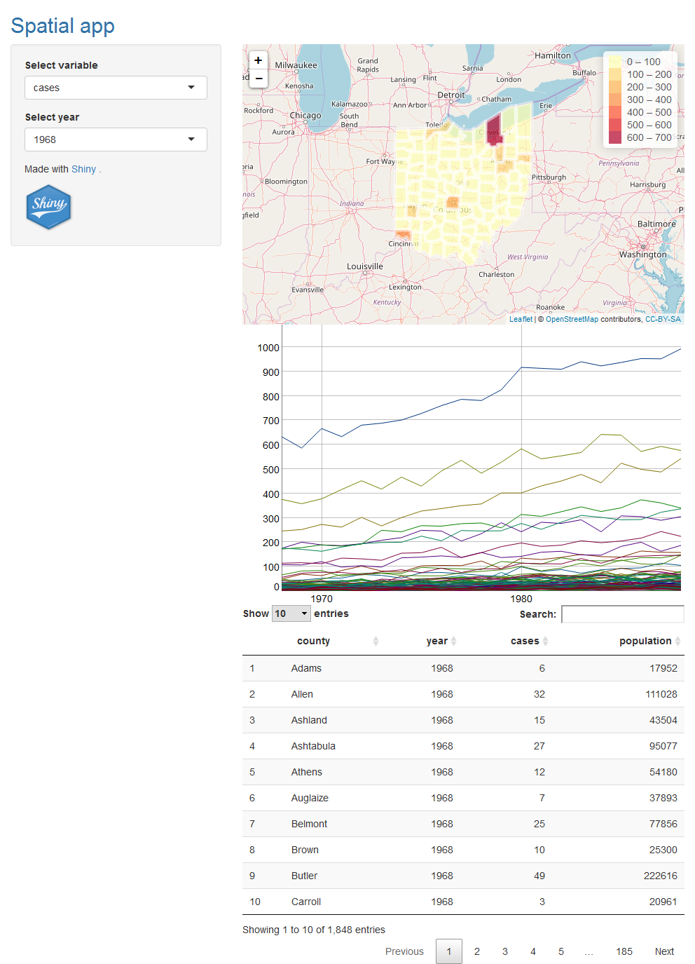
12 Upload data
Instead of reading the data files at the beginning of the app, we may want to upload our own files. In order to do that, we delete the code we previously used to read the data, and add two inputs that enable to upload a csv file and a shapefile.
12.1 Inputs in ui to upload a csv file and a shapefile
We create inputs to upload the data with the fileInput() function. fileInput() has a parameter called multiple that can be set to TRUE to allow the user to select multiple files. It also has a parameter called accept that can be set to a character vector with the type of files the input expects.
Here we write two inputs. One of the inputs is to upload the data. This input has name filedata and the input value can be accessed with input$filedata. This input accepts .csv files.
# in ui
fileInput(inputId = "filedata", label = "Upload data. Choose csv file",
          accept = c(".csv")),
The other input is to upload the shapefile. This input has name filemap and the input value can be accessed with input$filemap. This input accepts multiple files of type '.shp','.dbf','.sbn','.sbx','.shx', and '.prj'.
# in ui
fileInput(inputId = "filemap", label = "Upload map. Choose shapefile",
          multiple = TRUE, accept = c('.shp','.dbf','.sbn','.sbx','.shx','.prj')),
Note that a shapefile consist of different files with extensions .shp, .dbf, .shx etc. When we are using the Shiny app and uploading the shapefile, we need to upload all these files at once. That is, we need to select all the files and then click upload. Selecting just the file with extension .shp does not upload the shapefile.
12.2 Upload csv file in server()
We use the input values to read the csv file and the shapefile. We do this within a reactive expression. A reactive expression is an R expression that uses an input value and returns a value. To create a reactive expression we use the reactive() function, which takes an R expression surrounded by braces ({}). The reactive expression updates whenever the input value changes.
For example, we read the data with read.csv(input$filedata$datapath) where input$filedata$datapath is the data path contained in the value of the input that uploads the data. We put read.csv(input$filedata$datapath) inside reactive(). In this way, each time input$filedata$datapath is updated, the reactive expression is re-executed. The output of the reactive expression is assigned to data. In server(), data can be accessed with data(). data() will be updated each time the reactive expression that builds is re-executed.
# in server()
data <- reactive({read.csv(input$filedata$datapath)})
12.3 Upload shapefile in server()
We also write a reactive expression to read the map. We assign the result of the reactive expression to map. In server(), we access the map with map().
To read the shapefile we use the readOGR() function of the rgdal package. When files are uploaded with fileInput() they have different names from the ones in the directory. We first rename files with the actual names and then read the shapefile with readOGR() passing the name of the file with .shp extension.
# in server()
map <- reactive({
  # shpdf is a data.frame with the name, size, type and datapath of the uploaded files
  shpdf <- input$filemap

  # The files are uploaded with names 0.dbf, 1.prj, 2.shp, 3.xml, 4.shx
  # (path/names are in column datapath)
  # We need to rename the files with the actual names: fe_2007_39_county.dbf, etc.
  # (these are in column name)

  # Name of the temporary directory where files are uploaded
  tempdirname <- dirname(shpdf$datapath[1])

  # Rename files
  for(i in 1:nrow(shpdf)){
    file.rename(shpdf$datapath[i], paste0(tempdirname, "/", shpdf$name[i]))
  }

  # Now we read the shapefile with readOGR() of rgdal package
  # passing the name of the file with .shp extension.

  # We use the function grep() to search the pattern "*.shp$"
  # within each element of the character vector shpdf$name.
  # grep(pattern="*.shp$", shpdf$name)
  # ($ at the end denote files that finish with .shp, not only that contain .shp)
  map <- readOGR(paste(tempdirname, shpdf$name[grep(pattern = "*.shp$", shpdf$name)], sep = "/"))
  map
})
12.4 Access the data and the map
To access the data and the map in renderDT(), renderLeaflet() and renderDygraph(), we use map() and data().
#in server()

output$table <- renderDT(data())

output$map <- renderLeaflet({
map <- map()
data <- data()
...
})


output$timetrend <- renderDygraph({
data <- data()
...
})
13 Content of app.R
The content of app.R is shown below.
library(shiny)
library(rgdal)
library(DT)
library(dygraphs)
library(xts)
library(leaflet)

# ui object
ui <- fluidPage(
  titlePanel(p("Spatial app", style = "color:#3474A7")),
  sidebarLayout(
    sidebarPanel(

      fileInput(inputId = "filedata", label = "Upload data. Choose csv file",
                accept = c(".csv")),
      fileInput(inputId = "filemap", label = "Upload map. Choose shapefile",
                multiple = TRUE, accept = c('.shp','.dbf','.sbn','.sbx','.shx','.prj')),

      selectInput(inputId = "variableselected", label = "Select variable",
                  choices = c("cases", "population")),
      selectInput(inputId = "yearselected", label = "Select year",
                  choices = 1968:1988),

      p("Made with", a("Shiny", href = "http://shiny.rstudio.com"), "."),
      img(src = "imageShiny.png", width = "70px", height = "70px")
    ),

    mainPanel(
      leafletOutput(outputId = "map"),
      dygraphOutput(outputId = "timetrend"),
      DTOutput(outputId = "table")
    )
  )
)

# server()
server <- function(input, output){
  data <- reactive({read.csv(input$filedata$datapath)})

  map <- reactive({
    # shpdf is a data.frame with the name, size, type and datapath of the uploaded files
    shpdf <- input$filemap

    # The files are uploaded with names 0.dbf, 1.prj, 2.shp, 3.xml, 4.shx
    # (path/names are in column datapath)
    # We need to rename the files with the actual names: fe_2007_39_county.dbf, etc.
    # (these are in column name)

    # Name of the temporary directory where files are uploaded
    tempdirname <- dirname(shpdf$datapath[1])

    # Rename files
    for(i in 1:nrow(shpdf)){
      file.rename(shpdf$datapath[i], paste0(tempdirname, "/", shpdf$name[i]))
    }

    # Now we read the shapefile with readOGR() of rgdal package
    # passing the name of the file with .shp extension.

    # We use the function grep() to search the pattern "*.shp$"
    # within each element of the character vector shpdf$name.
    # grep(pattern="*.shp$", shpdf$name)
    # ($ at the end denote files that finish with .shp, not only that contain .shp)
    map <- readOGR(paste(tempdirname, shpdf$name[grep(pattern = "*.shp$", shpdf$name)], sep ="/"))
    map
  })

  output$table <- renderDT(data())

  output$timetrend <- renderDygraph({
    data <- data()

    dataxts <- NULL
    counties <- unique(data$county)
    for(l in 1:length(counties)){
      datacounty <- data[data$county == counties[l],]
      dd <- xts(datacounty[, input$variableselected], as.Date(paste0(datacounty$year,"-01-01")))
      dataxts <- cbind(dataxts, dd)
    }
    colnames(dataxts) <- counties

    dygraph(dataxts) %>% dyHighlight(highlightSeriesBackgroundAlpha = 0.2)-> d1

    d1$x$css = "
 .dygraph-legend > span {display:none;}
 .dygraph-legend > span.highlight { display: inline; }
 "
    d1
  })

  output$map <- renderLeaflet({
    map <- map()
    data <- data()

    # Add data to map
    datafiltered <- data[which(data$year == input$yearselected), ]
    ordercounties <- match(map@data$NAME, datafiltered$county)
    map@data <- datafiltered[ordercounties, ]

    # Create variableplot
    map$variableplot <- as.numeric(map@data[, input$variableselected])

    # Create leaflet
    pal <- colorBin("YlOrRd", domain = map$variableplot, bins = 7)

    labels <- sprintf("%s: %g", map$county, map$variableplot) %>% lapply(htmltools::HTML)

    l <- leaflet(map) %>% addTiles() %>% addPolygons(
      fillColor = ~pal(variableplot),
      color = "white",
      dashArray = "3",
      fillOpacity = 0.7,
      label = labels) %>%
      leaflet::addLegend(pal = pal, values = ~variableplot, opacity = 0.7, title = NULL)
  })
}

# shinyApp()
shinyApp(ui = ui, server = server)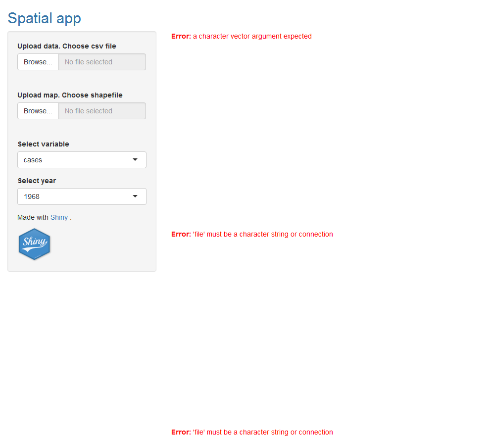
14 Handle missing inputs
14.1 Require input files to be available using req()
We note that until the user upload the files the outputs render error messages. Here we add code that makes the output not to be shown until the data is uploaded. We do this by using inside the reactive expression the function req(input$inputId) that means require input$inputId to be available. req() evaluates its arguments one at a time and if these are missing it stops. In this way, the value returned by the reactive expression will not be updated, and outputs that use the value returned by the reactive expression will not be re-executed. Details on how to use req() are here.
We add req(input$filedata) at the beginning of the reactive expression that reads the data. If the data has not been uploaded yet, input$filedata is equal to "". This makes the execution of the reactive expression stop, data() is not updated, and the output depending on data() is not executed.
# in ui. First line in the reactive() that reads the data
req(input$filedata)
Similarly, we add req(input$filemap) at the beginning of the reactive expression that reads the map. If the map has not been uploaded yet, input$filemap is missing, the execution of the reactive expression stops, map() is not updated, and the output depending on map() is not executed.
# in ui. First line in the reactive() that reads the map
req(input$filemap)
14.2 Check both the data and the shapefile are uploaded before plotting the leaflet map
Before constructing the leaflet map, the data has to be added to the shapefile. To do this we need to make sure that both the data and the map are uploaded. We can do this by writing at the beginning of renderLeaflet() the following code.
output$map <- renderLeaflet({
  if(is.null(data()) | is.null(map())){
    return(NULL)
  }
  ...
})
When either data() or map() are updated, the instructions of renderLeaflet() are executed. Then, at the beginning of renderLeaflet() it is checked whether either data() or map() are NULL. If this is TRUE, the execution stops returning NULL. This avoids the error that we would get when trying to add the data to the map when either of these two elements are NULL.
15 Content of app.R
The complete code of app.R is given below.
library(shiny)
library(rgdal)
library(DT)
library(dygraphs)
library(xts)
library(leaflet)

# ui object
ui <- fluidPage(
  titlePanel(p("Spatial app", style = "color:#3474A7")),
  sidebarLayout(
    sidebarPanel(
      fileInput(inputId = "filedata", label = "Upload data. Choose csv file",
                accept = c(".csv")),
      fileInput(inputId = "filemap", label = "Upload map. Choose shapefile",
                multiple = TRUE, accept=c('.shp','.dbf','.sbn','.sbx','.shx','.prj')),
      selectInput(inputId = "variableselected", label = "Select variable",
                  choices = c("cases", "population")),
      selectInput(inputId = "yearselected", label = "Select year",
                  choices = 1968:1988),
      p("Made with", a("Shiny", href = "http://shiny.rstudio.com"), "."),
      img(src = "imageShiny.png", width = "70px", height = "70px")
    ),

    mainPanel(
      leafletOutput(outputId = "map"),
      dygraphOutput(outputId = "timetrend"),
      DTOutput(outputId = "table")
    )
  )
)

# server()
server <- function(input, output){
  data <- reactive({
    req(input$filedata)
    read.csv(input$filedata$datapath)})

  map <- reactive({
    req(input$filemap)

    # shpdf is a data.frame with the name, size, type and datapath of the uploaded files
    shpdf <- input$filemap

    # The files are uploaded with names 0.dbf, 1.prj, 2.shp, 3.xml, 4.shx
    # (path/names are in column datapath)
    # We need to rename the files with the actual names: fe_2007_39_county.dbf, etc.
    # (these are in column name)

    # Name of the temporary directory where files are uploaded
    tempdirname <- dirname(shpdf$datapath[1])

    # Rename files
    for(i in 1:nrow(shpdf)){
      file.rename(shpdf$datapath[i], paste0(tempdirname, "/", shpdf$name[i]))
    }

    # Now we read the shapefile with readOGR() of rgdal package
    # passing the name of the file with .shp extension.

    # We use the function grep() to search the pattern "*.shp$"
    # within each element of the character vector shpdf$name.
    # grep(pattern="*.shp$", shpdf$name)
    # ($ at the end denote files that finish with .shp, not only that contain .shp)
    map <- readOGR(paste(tempdirname, shpdf$name[grep(pattern = "*.shp$", shpdf$name)], sep="/"))
    map
  })

  output$table <- renderDT(data())

  output$timetrend <- renderDygraph({
    data <- data()
    dataxts <- NULL
    counties <- unique(data$county)
    for(l in 1:length(counties)){
      datacounty <- data[data$county == counties[l],]
      dd <- xts(datacounty[, input$variableselected], as.Date(paste0(datacounty$year,"-01-01")))
      dataxts <- cbind(dataxts, dd)
    }
    colnames(dataxts) <- counties
    dygraph(dataxts) %>% dyHighlight(highlightSeriesBackgroundAlpha = 0.2)-> d1
    d1$x$css = "
 .dygraph-legend > span {display:none;}
 .dygraph-legend > span.highlight { display: inline; }
 "
    d1
  })

  output$map <- renderLeaflet({
    if(is.null(data()) | is.null(map())){
      return(NULL)
    }

    map <- map()
    data <- data()

    # Add data to map
    datafiltered <- data[which(data$year == input$yearselected), ]
    ordercounties <- match(map@data$NAME, datafiltered$county)
    map@data <- datafiltered[ordercounties, ]

    # Create variableplot
    map$variableplot <- as.numeric(map@data[, input$variableselected])

    # Create leaflet
    pal <- colorBin("YlOrRd", domain = map$variableplot, bins = 7)
    labels <- sprintf("%s: %g", map$county, map$variableplot) %>% lapply(htmltools::HTML)

    l <- leaflet(map) %>% addTiles() %>% addPolygons(
      fillColor = ~pal(variableplot),
      color = "white",
      dashArray = "3",
      fillOpacity = 0.7,
      label = labels) %>%
      leaflet::addLegend(pal = pal, values = ~variableplot, opacity = 0.7, title = NULL)
  })
}

# shinyApp()
shinyApp(ui = ui, server = server)
16 Conclusion
In this tutorial we have shown how to build a Shiny app to visualize spatial and spatio-temporal data. We have seen how to include interactive visualizations: a DT table, a leaflet map and a dygraphs time series plot. We have also shown how to upload specific files and how to add functionality that enable the user to select specific information to be shown. We can also improve the appearance and functionality of the app by modifying the layout and adding different inputs and outputs with new functionality. Section References contains links to tutorials and R packages that can be used to improve the app.
17 References
- RStudio
Shinytutorial https://shiny.rstudio.com/tutorial/written-tutorial/lesson1/ Shinyhttps://shiny.rstudio.com/.DThttps://rstudio.github.io/DT/dygraphshttps://rstudio.github.io/dygraphs/leaflethttps://rstudio.github.io/leaflet/SpatialEpiApphttps://paula-moraga.github.io/software/

This work by Paula Moraga is licensed under a Creative Commons Attribution-NonCommercial-ShareAlike 4.0 International License.