Analysis of data using Seurat package, similar to tutorial at: http://satijalab.org/seurat/pbmc3k_tutorial.html.

For the tutorial below, we will use human tonsil innate lymphoid cells (ILCs) example dataset from Björklund et. al., 2016. But you can also run with your own data. But keep in mind that some functions assume that the count data is UMIs, but we run it with data from Smartseq2 using raw counts.

All data can be accessed here.

1 Load data

For running Seurat we need the metadata table, the count matrix and a file with gene name translations.

C <- read.table("ensembl_countvalues_ILC.csv",sep=",",header=T,row.names=1)
M <- read.table("Metadata_ILC.csv",sep=",",header=T,row.names=1)

# in this case it may be wise to translate ensembl IDs to gene names 
# to make plots with genes more understandable
# Read in gene name translations. 
TR <- read.table("gene_name_translation_biotype.tab",sep="\t")

# find the correct entries in TR and merge ensembl name and gene id.
m <- match(rownames(C),TR$ensembl_gene_id)
newnames <- apply(cbind(as.vector(TR$external_gene_name)[m],rownames(C)),1,paste,collapse=":")
rownames(C)<-newnames

2 Create Seurat object

Load packages:

suppressMessages(require(Seurat))
suppressMessages(require(gridExtra))

Seurat will automatically filter out genes/cells that do not meet the criteria specified to save space. The cutoffs are defined with min.cells and min.genes . However, in this case, the cells are already filtered, but all genes that are not expressed with >1 count in 3 cells (min.cells) will be removed.

# in seurat we will not make use of the spike-ins, so remove them from the expression matrix before creating the Seurat object. 
ercc <- grep("ERCC_",rownames(C))

# Create the Seurat object.
data <- CreateSeuratObject(raw.data = C[-ercc,], 
                           min.cells = 3, min.genes = 200, 
                           project = "ILC", is.expr=1, meta.data=M)

3 The Seurat object

The Seurat object you have created now contains several slots with different information.

slotNames(data)

##  [1] "raw.data"     "data"         "scale.data"   "var.genes"   
##  [5] "is.expr"      "ident"        "meta.data"    "project.name"
##  [9] "dr"           "assay"        "hvg.info"     "imputed"     
## [13] "cell.names"   "cluster.tree" "snn"          "calc.params" 
## [17] "kmeans"       "spatial"      "misc"         "version"

Some of the most important ones to know are:

raw.data - the raw input (counts)
data - the normalized and log-transformed data
scale.data - the scaled data
var.genes - the variable genes
hvg.info - the mean and dispersion of all genes
dr - dimensionality reduction such as pca, tsne
ident - the default identity class used for coloring in all plots
meta.data - the meta data table.

4 Data overview

There are multiple functions in Seurat to visualize QC-data for your dataset. Below are some examples:

Violin plot for number of detected genes per cell.

# plot number of genes and nUMI (rpkms in this case) for each Donor
VlnPlot(object = data, features.plot = c("nGene", "nUMI"), nCol = 2, group.by = "Donor")

# same for celltype
VlnPlot(object = data, features.plot = c("nGene", "nUMI"), nCol = 2, group.by = "Celltype")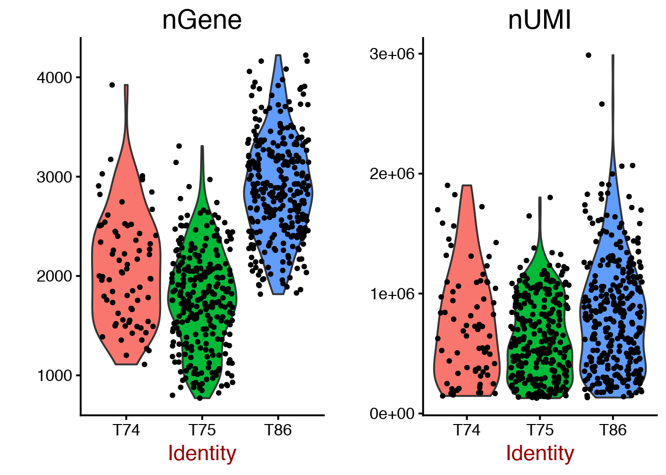

Scatterplot with detected genes vs Counts (not UMIs as it will say in the legend) since this is not UMI data.

GenePlot(object = data, gene1 = "nUMI", gene2 = "nGene")

The slot data@ident defines the grouping of cells, which is automatically set to Donor in this case. To instead color by celltype, data@ident needs to be changed.

data <- SetAllIdent(object = data, id = "Celltype")
GenePlot(object = data, gene1 = "nUMI", gene2 = "nGene")

# change ident back to Donor
data <- SetAllIdent(object = data, id = "Donor")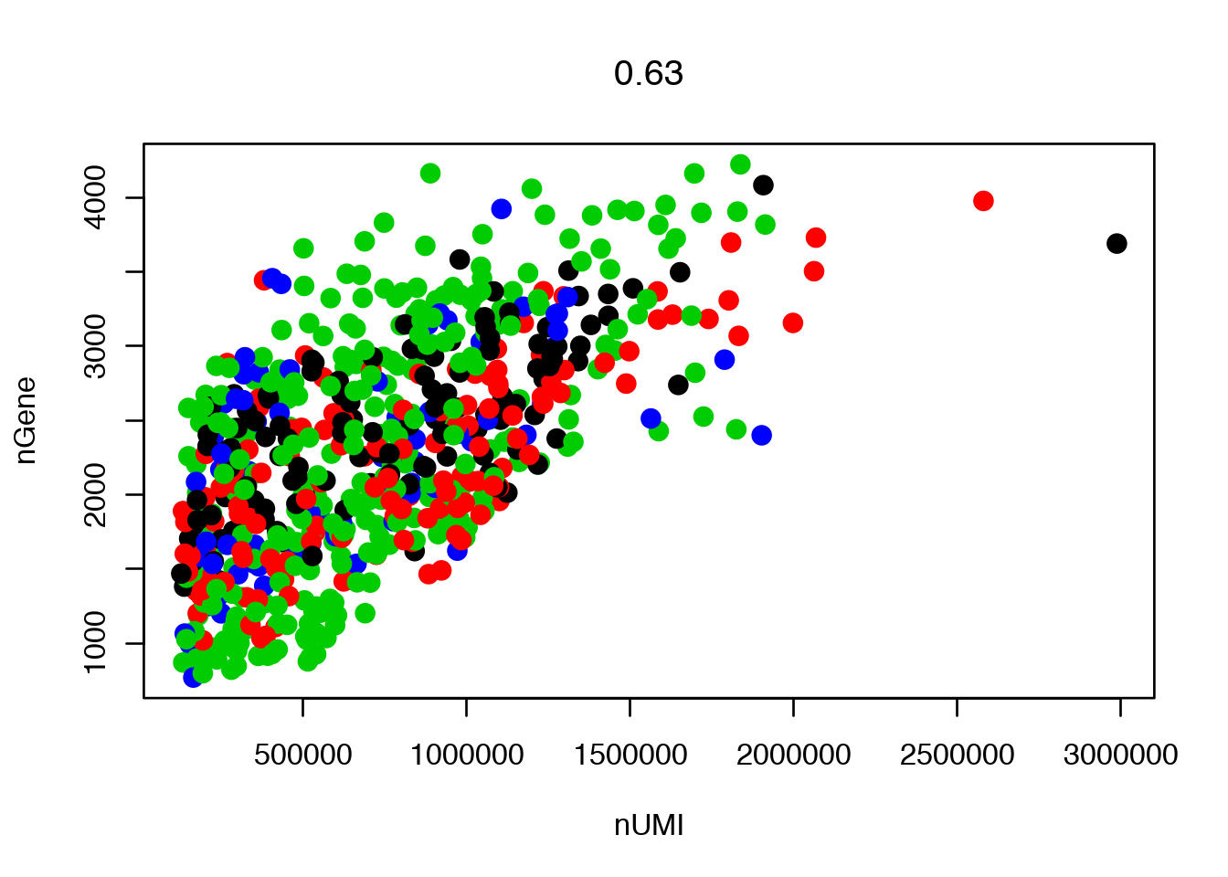

OBS! Each time you want to change colors in a gene plot, you need to change the identity class value in the seurat object in the slot data@ident. Perhaps there is a better way, but I did not find a solution.

In many of the other Seurat plotting functions like TSNEPlot(), PCAPlot() and VlnPlot(), you can use group.by to define which meta data variable the cells should be coloured or grouped by.

5 Data normalization and scaling

Next step is to normalize the data, detect variable genes and to scale the data.

5.1 Normalize

Normalize the data, converts to counts per million and log-transform it.

data <- NormalizeData(object = data, normalization.method = "LogNormalize")

5.2 Find variable genes

You should look at the plot for suitable cutoffs for your specific dataset rerun the command. You can define the lower/upper bound of mean expression with x.low.cutoff/x.high.cutoff and the limit of dispersion with y.cutoff

data <- FindVariableGenes(object = data, mean.function = ExpMean, dispersion.function = LogVMR, x.low.cutoff = 0.5, x.high.cutoff = 10, y.cutoff = 0.5)

length(x = data@var.genes)

## [1] 838

5.3 Scale the data

Scales and centers genes in the dataset. The scaling step can also be used to remove unwanted confounders.

It is quite common to regress out the number of detected genes (nGene), that quite often will drive the variation in your data due to library quality.

We will also run one version of scaling where we include the Donor batch information and compare.

data <- ScaleData(object = data, vars.to.regress = c("nGene"), display.progress=F)

# also with batch info + detected genes.
dataB <- ScaleData(object = data, vars.to.regress = c("nGene","Donor"), display.progress=F)

6 PCA

Run PCA using variable genes. The pca is stored in the slot dr.

# run PCA for both objects
data <- RunPCA(object = data, pc.genes = data@var.genes, do.print = FALSE)
dataB <- RunPCA(object = dataB, pc.genes = data@var.genes, do.print = FALSE)

Vizualize gene loadings

VizPCA(object = data, pcs.use = 1:4)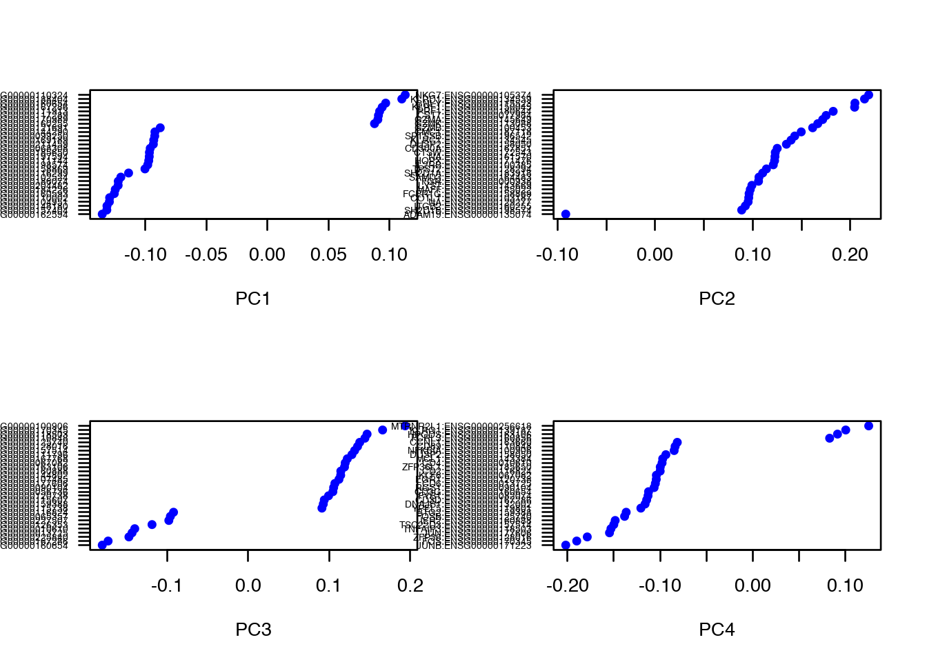

Plot PCA for both objects. To put multiple plots in the same window, do.return=T was used to return the ggplot2 objects and that are plotted in one window with grid.arrange.

p1 <- PCAPlot(object = data, dim.1 = 1, dim.2 = 2, do.return=T, plot.title = "Uncorrected")
p2 <- PCAPlot(object = dataB, dim.1 = 1, dim.2 = 2, do.return=T, plot.title = "Batch corrected")

# and with both color by Celltype, here you can use group.by 
p3 <- PCAPlot(object = data, dim.1 = 1, dim.2 = 2, do.return=T,group.by="Celltype", plot.title = "Uncorrected")
p4 <- PCAPlot(object = dataB, dim.1 = 1, dim.2 = 2, do.return=T,group.by="Celltype", plot.title = "Batch corrected")

# plot together
grid.arrange(p1,p2,p3,p4,ncol=2)

As you can see, the batch effect is not as strong in this PCA as it was in PCAs that we did in other labs, so the PCA plot with batch correction does look quite similar.

This is mainly due to the fact that we are only using top variable genes, and it seems that the batch effect is mainly seen among genes that are not highly variable.

Still, if you know you have a clear batch effect, it is a good idea to remove it with regression. So from now on, we will continue with the dataB object.

6.1 Heatmap with top loading genes

OBS! Margins are too large to display well in R-studio, save to a pdf instead.

pdf("seurat_pc_loadings_heatmaps.pdf")
PCHeatmap(object = dataB, pc.use = 1, do.balanced = TRUE, label.columns = FALSE)
PCHeatmap(object = dataB, pc.use = 1:5, do.balanced = TRUE, label.columns = FALSE)
dev.off()

## pdf 
##   2

6.2 Determine statistically significant principal components

Now we use the JackStraw function to check which of the principal components that are significant. If dataset is large, you can instead use PCElbowPlot().

As a default, JackStraw is only run on the first 20 PCs, if you want to include more PCs in your tSNE and clustering, run JackStraw with num.pc=30 or similar.

dataB <- JackStraw(object = dataB, num.replicate = 100,display.progress =F)
JackStrawPlot(object = dataB, PCs = 1:12)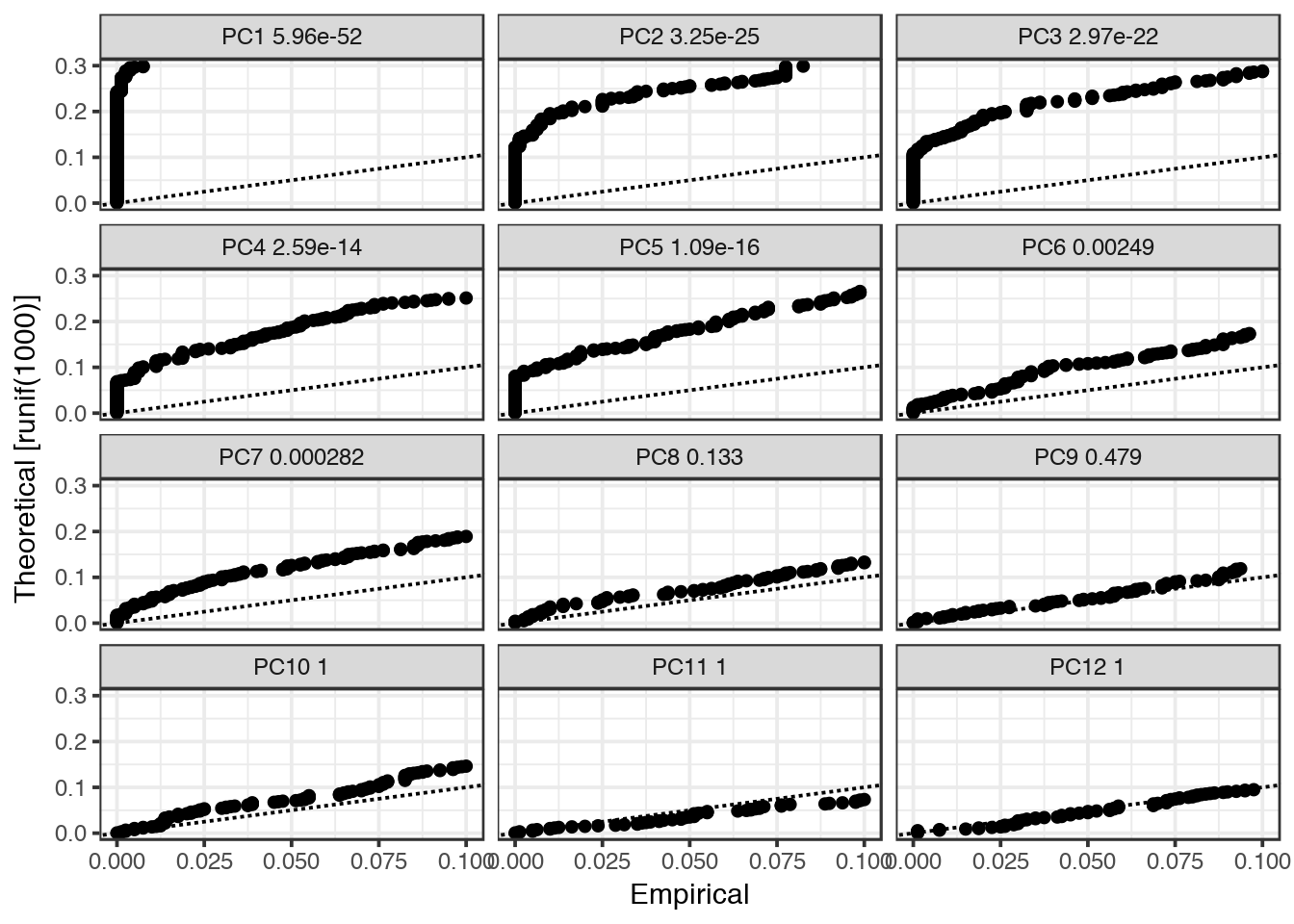

In this case, only PCs 1-7 are significant, so we will only use those in subsequent steps.

7 Find clusters

In this case, we use the PCs as suggested by the JackStrawPlot(). FindClusters() constructs a SNN-graph based on distances in PCA space using the defined principal components. This graph is split into clusters using modularity optimization techniques.

You can tweak the clustering with the resolution parameter to get more/less clusters and also with parameters k and k.scale for the construction of the graph.

OBS! Any function that depends on random start positions, like the KNN graph and tSNE will not give identical results each time you run it. So it is adviced to set the random seed with set.seed function before running the function.

use.pcs <- 1:7
set.seed(1)
dataB <- FindClusters(object = dataB, reduction.type = "pca", dims.use = use.pcs, resolution = 0.6, print.output = 0, save.SNN = TRUE)

PrintFindClustersParams(object = dataB)

## Parameters used in latest FindClusters calculation run on: 2018-06-15 21:26:08
## =============================================================================
## Resolution: 0.6
## -----------------------------------------------------------------------------
## Modularity Function    Algorithm         n.start         n.iter
##      1                   1                 100             10
## -----------------------------------------------------------------------------
## Reduction used          k.param          prune.SNN
##      pca                 30                0.0667
## -----------------------------------------------------------------------------
## Dims used in calculation
## =============================================================================
## 1 2 3 4 5 6 7

After doing clustering, the slot data@ident will automatically change to the cluster definition.

8 tSNE

For visualization, we use a tSNE with the same PCs as in the clustering.

set.seed(1)
dataB <- RunTSNE(object = dataB, dims.use = use.pcs, do.fast = TRUE)

# note that you can set do.label=T to help label individual clusters
TSNEPlot(object = dataB,do.label = T)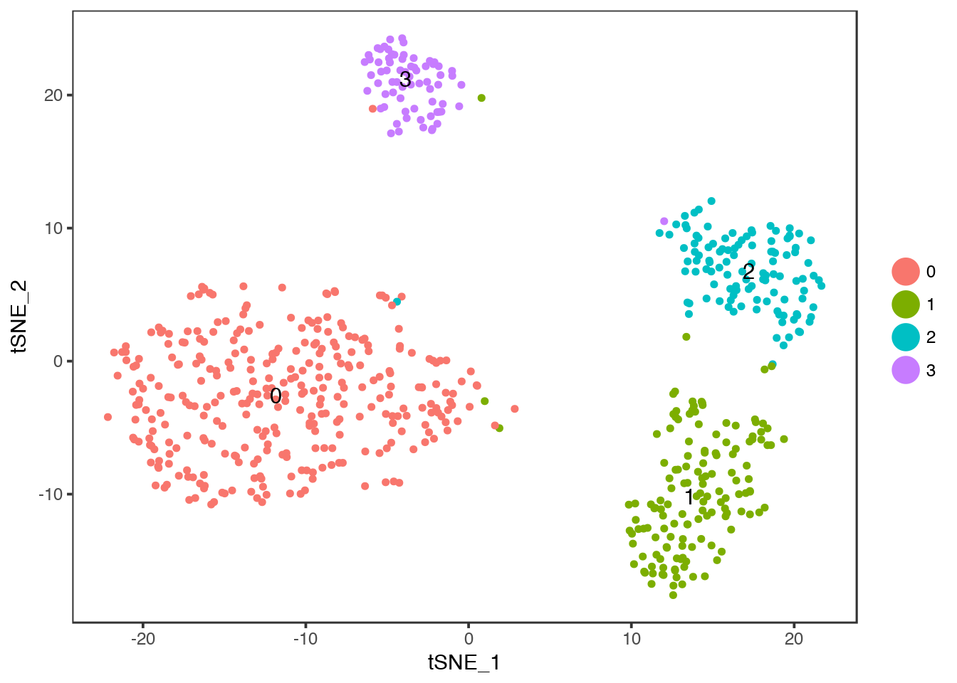

Compare to celltype identities, colour instead by Celltype with group.by.

TSNEPlot(object = dataB, group.by = "Celltype")

Colour instead by Donor.

TSNEPlot(object = dataB, group.by = "Donor")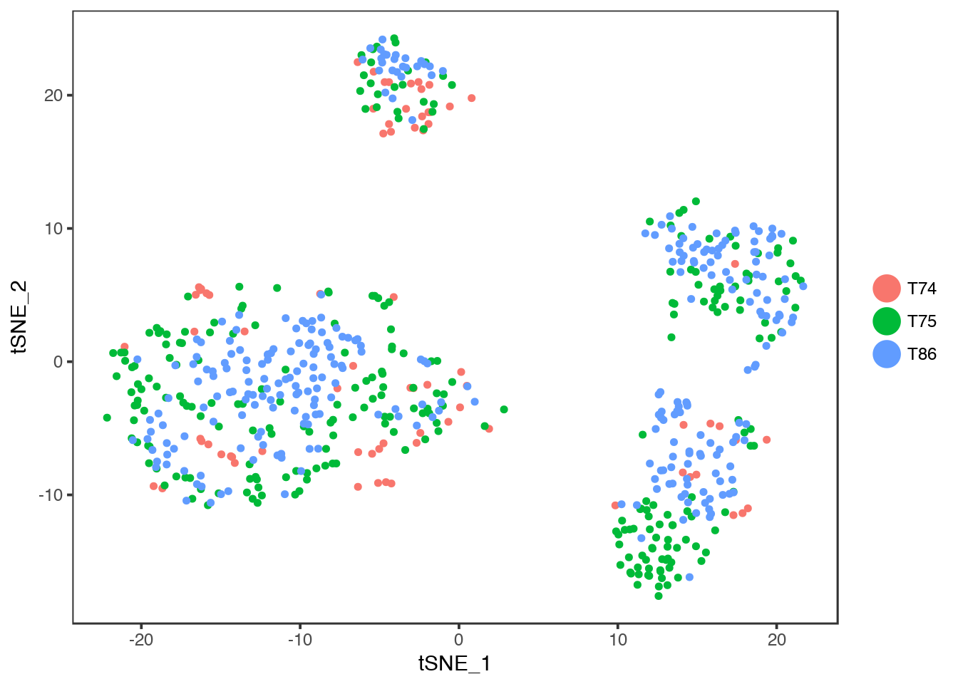

9 Cluster markers

Now we can find and plot some of the cluster markers to check if our clustering makes sense. The default method in Seurat is a Wilcoxon rank sum test. The Differential expression tests that are implemented in Seurat are:

wilcox : Wilcoxon rank sum test (default)
bimod : Likelihood-ratio test for single cell gene expression (McDavid et al., Bioinformatics, 2013).
roc : Standard AUC classifier
t : Student’s t-test
tobit : Tobit-test for differential gene expression (Trapnell et al., Nature Biotech, 2014).
poisson : Likelihood ratio test assuming an underlying poisson distribution. Use only for UMI-based datasets
negbinom : Likelihood ratio test assuming an underlying negative binomial distribution. Use only for UMI-based datasets
MAST : GLM-framework that treates cellular detection rate as a covariate (Finak et al, Genome Biology, 2015).
DESeq2 : DE based on a model using the negative binomial distribution (Love et al, Genome Biology, 2014).

# find all genes that defines cluster1, we compare cluster1 to all the other clusters. 
cluster1.markers <- FindMarkers(object = dataB, ident.1 = 1, min.pct = 0.25)
print(head(cluster1.markers),5)

##                               p_val  avg_logFC pct.1 pct.2    p_val_adj
## HPGDS:ENSG00000163106  1.030886e-71  1.4132524 0.614 0.016 2.576700e-67
## CD2:ENSG00000116824    9.106426e-62 -2.4299716 0.221 0.942 2.276151e-57
## PTGDR2:ENSG00000183134 1.355328e-58  1.1848458 0.503 0.010 3.387643e-54
## KRT1:ENSG00000167768   9.555356e-58  1.7732377 0.552 0.028 2.388361e-53
## IL17RB:ENSG00000056736 3.051531e-54  1.8174596 0.614 0.062 7.627301e-50
## FSTL4:ENSG00000053108  2.005269e-50  0.9605111 0.497 0.024 5.012171e-46

As you can see, some of the genes are higher in cluster1, and have a positive fold change (avg_logFC) while others are lower in cluster1 such as CD2.

Plot top cluster1 markers as violins.

VlnPlot(object = dataB, features.plot = rownames(cluster1.markers)[1:6],nCol=3,size.title.use=10)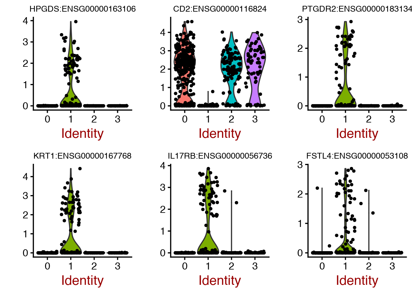

Plot them on to the tSNE layout.

FeaturePlot(object = dataB, features.plot = rownames(cluster1.markers)[1:6], cols.use = c("yellow", "red","black"), reduction.use = "tsne")

And as a ridge plot.

RidgePlot(object = dataB, features.plot = rownames(cluster1.markers)[1:6])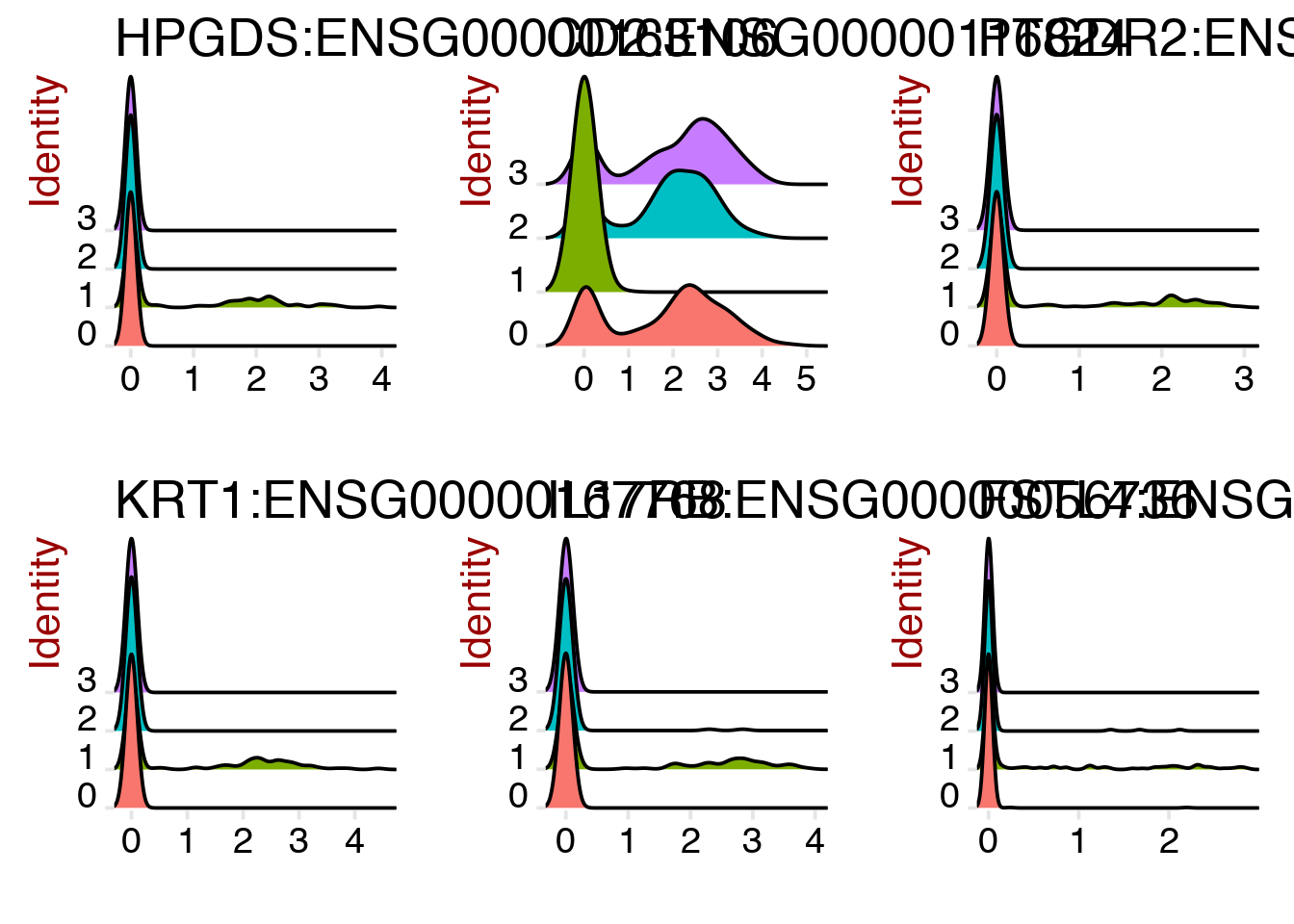

You can also specify specific cells, or clusters that you want to compare:

# find genes that separates cluster 0 & cluster 3 by specifying both ident.1 and ident.2 
cluster03.markers <- FindMarkers(object = dataB, ident.1 = 0, ident.2 = 3, min.pct = 0.25)
print(x = head(x = cluster03.markers, n = 5))

##                              p_val avg_logFC pct.1 pct.2    p_val_adj
## NKG7:ENSG00000105374  2.197786e-47 -2.874669 0.250 0.971 5.493366e-43
## KLRD1:ENSG00000134539 1.490071e-45 -2.786882 0.262 0.971 3.724431e-41
## KLRF1:ENSG00000150045 1.667989e-39 -2.456823 0.209 0.871 4.169138e-35
## CST7:ENSG00000077984  1.498830e-38 -1.744451 0.122 0.800 3.746325e-34
## PRF1:ENSG00000180644  2.738346e-38 -2.562743 0.184 0.843 6.844495e-34

You can also run function FindAllMarkers() wich will run DE detection for all the clusters vs the rest (or any other classification you may have in the ident slot).

10 Extra tasks

Now you should be familiar with the basics of the Seurat package. If you still have time, we have suggestions for some extra exercises that you can perform:

Rerun the clustering step and see what happens when you change the settings for k.param and resolution. Can you tweak it to get more/less clusters?
Try out some of the other methods for differential expression that are implemented in Seurat. Do you get the same genes as with the Wilcoxon test?

11 Session Info

This document has been created in RStudio using R Markdown and related packages.
For R Markdown, see http://rmarkdown.rstudio.com
For details about the OS, packages and versions, see detailed information below:

sessionInfo()

## R version 3.4.3 (2017-11-30)
## Platform: x86_64-w64-mingw32/x64 (64-bit)
## Running under: Windows >= 8 x64 (build 9200)
## 
## Matrix products: default
## 
## locale:
## [1] LC_COLLATE=English_United Kingdom.1252 
## [2] LC_CTYPE=English_United Kingdom.1252   
## [3] LC_MONETARY=English_United Kingdom.1252
## [4] LC_NUMERIC=C                           
## [5] LC_TIME=English_United Kingdom.1252    
## 
## attached base packages:
## [1] stats     graphics  grDevices utils     datasets  methods   base     
## 
## other attached packages:
##  [1] bindrcpp_0.2.2  gridExtra_2.3   Seurat_2.3.1    Matrix_1.2-14  
##  [5] cowplot_0.9.2   forcats_0.3.0   stringr_1.3.1   dplyr_0.7.5    
##  [9] purrr_0.2.5     readr_1.1.1     tidyr_0.8.1     tibble_1.4.2   
## [13] ggplot2_2.2.1   tidyverse_1.2.1 captioner_2.2.3 bookdown_0.7   
## [17] knitr_1.20     
## 
## loaded via a namespace (and not attached):
##   [1] readxl_1.1.0         snow_0.4-2           backports_1.1.2     
##   [4] Hmisc_4.1-1          VGAM_1.0-5           plyr_1.8.4          
##   [7] igraph_1.2.1         lazyeval_0.2.1       splines_3.4.3       
##  [10] digest_0.6.15        foreach_1.4.4        htmltools_0.3.6     
##  [13] lars_1.2             gdata_2.18.0         magrittr_1.5        
##  [16] checkmate_1.8.5      cluster_2.0.7-1      mixtools_1.1.0      
##  [19] ROCR_1.0-7           sfsmisc_1.1-2        recipes_0.1.2       
##  [22] modelr_0.1.2         gower_0.1.2          dimRed_0.1.0        
##  [25] R.utils_2.6.0        colorspace_1.3-2     rvest_0.3.2         
##  [28] haven_1.1.1          xfun_0.1             crayon_1.3.4        
##  [31] jsonlite_1.5         bindr_0.1.1          zoo_1.8-2           
##  [34] survival_2.42-3      iterators_1.0.9      ape_5.1             
##  [37] glue_1.2.0           DRR_0.0.3            gtable_0.2.0        
##  [40] ipred_0.9-6          kernlab_0.9-26       ddalpha_1.3.3       
##  [43] prabclus_2.2-6       DEoptimR_1.0-8       abind_1.4-5         
##  [46] scales_0.5.0.9000    mvtnorm_1.0-8        Rcpp_0.12.17        
##  [49] metap_0.9            dtw_1.20-1           htmlTable_1.12      
##  [52] tclust_1.4-1         magic_1.5-8          reticulate_1.8      
##  [55] foreign_0.8-70       proxy_0.4-22         mclust_5.4          
##  [58] SDMTools_1.1-221     Formula_1.2-3        tsne_0.1-3          
##  [61] stats4_3.4.3         lava_1.6.1           prodlim_2018.04.18  
##  [64] htmlwidgets_1.2      httr_1.3.1           FNN_1.1             
##  [67] gplots_3.0.1         RColorBrewer_1.1-2   fpc_2.1-11          
##  [70] acepack_1.4.1        modeltools_0.2-21    ica_1.0-2           
##  [73] pkgconfig_2.0.1      R.methodsS3_1.7.1    flexmix_2.3-14      
##  [76] nnet_7.3-12          caret_6.0-80         labeling_0.3        
##  [79] tidyselect_0.2.4     rlang_0.2.1          reshape2_1.4.3      
##  [82] munsell_0.5.0        cellranger_1.1.0     tools_3.4.3         
##  [85] cli_1.0.0            ranger_0.10.1        ggridges_0.5.0      
##  [88] broom_0.4.4          evaluate_0.10.1      geometry_0.3-6      
##  [91] yaml_2.1.19          ModelMetrics_1.1.0   fitdistrplus_1.0-9  
##  [94] robustbase_0.93-0    caTools_1.17.1       RANN_2.5.1          
##  [97] pbapply_1.3-4        nlme_3.1-137         R.oo_1.22.0         
## [100] RcppRoll_0.3.0       xml2_1.2.0           compiler_3.4.3      
## [103] rstudioapi_0.7       png_0.1-7            stringi_1.2.3       
## [106] lattice_0.20-35      trimcluster_0.1-2    psych_1.8.4         
## [109] diffusionMap_1.1-0   pillar_1.2.3         lmtest_0.9-36       
## [112] irlba_2.3.2          data.table_1.11.4    bitops_1.0-6        
## [115] R6_2.2.2             latticeExtra_0.6-28  KernSmooth_2.23-15  
## [118] codetools_0.2-15     MASS_7.3-50          gtools_3.5.0        
## [121] assertthat_0.2.0     CVST_0.2-2           rprojroot_1.3-2     
## [124] withr_2.1.2          mnormt_1.5-5         diptest_0.75-7      
## [127] parallel_3.4.3       doSNOW_1.0.16        hms_0.4.2           
## [130] grid_3.4.3           rpart_4.1-13         timeDate_3043.102   
## [133] class_7.3-14         rmarkdown_1.10       segmented_0.5-3.0   
## [136] Cairo_1.5-9          Rtsne_0.13           scatterplot3d_0.3-41
## [139] lubridate_1.7.4      base64enc_0.1-3

Page built on: 15-Jun-2018 at 21:26:40.

2018 | SciLifeLab > NBIS > RaukR

Hands-On using Seurat

scRNA-Seq Analysis

Åsa Björklund

15-Jun-2018