1 Prepare data

suppressMessages(library(scater))

# read in meta data table and create pheno data
M <- read.table("data/ILC/Metadata_ILC.csv", sep=",",header=T)

# read the count matrix
C <- read.table("data/ILC/ensembl_countvalues_ILC.csv",sep=",",header=T)

head(M)

2 Create the SCESet

# create an SCESet using the counts in C and the metadata in M
sce <- SingleCellExperiment(assays = list(counts = as.matrix(C)), colData = M)

# the function normalize will divide by size factors and log-transform. 
sce <- normalize(sce)

Normalization can be performed with other size factors than total counts using the scran package.

We have accessor functions to access elements of the SingleCellExperiment object.

• counts(object): returns the matrix of read counts. If no counts are defined for the object, then the counts matrix slot is simpy NULL.

• exprs(object): returns the matrix of (log-counts) expression values, in fact accessing the logcounts slot of the object (synonym for logcounts).

For convenience (and backwards compatibility with SCESet) getters and setters are provided as follows: exprs, tpm, cpm, fpkm and versions of these with the prefix “norm_”)

# you can access the rpkm or count matrix with the commands "counts" and "exprs"
counts(sce)[10:13,1:5]
exprs(sce)[10:13,1:5]

##                 T74_P1_A9_ILC1 T74_P1_B4_NK T74_P1_B7_ILC2 T74_P1_B9_NK
## ENSG00000001167              0            0              0            0
## ENSG00000001460              0            0              0            0
## ENSG00000001461              0         1035              1            1
## ENSG00000001497              0            0              0            0
##                 T74_P1_D10_ILC2
## ENSG00000001167               0
## ENSG00000001460               0
## ENSG00000001461               2
## ENSG00000001497               0
##                 T74_P1_A9_ILC1 T74_P1_B4_NK T74_P1_B7_ILC2 T74_P1_B9_NK
## ENSG00000001167              0     0.000000       0.000000    0.0000000
## ENSG00000001460              0     0.000000       0.000000    0.0000000
## ENSG00000001461              0     8.633496       0.750417    0.7430397
## ENSG00000001497              0     0.000000       0.000000    0.0000000
##                 T74_P1_D10_ILC2
## ENSG00000001167        0.000000
## ENSG00000001460        0.000000
## ENSG00000001461        2.063469
## ENSG00000001497        0.000000

The SCE object also has slots for:

• colData - cell metadata, which can be supplied as a DataFrame object, where rows are cells, and columns are cell attributes (such as cell type, culture condition, day captured, etc.).
• rowData - feature metadata, which can be supplied as a DataFrame object, where rows are features (e.g. genes), and columns are feature attributes, such as Ensembl ID, biotype, gc content, etc.

head(colData(sce))

head(rowData(sce))

## DataFrame with 6 rows and 4 columns
##                         Samples    Plate    Donor Celltype
##                        <factor> <factor> <factor> <factor>
## T74_P1_A9_ILC1   T74_P1_A9_ILC1   T74_P1      T74     ILC1
## T74_P1_B4_NK       T74_P1_B4_NK   T74_P1      T74       NK
## T74_P1_B7_ILC2   T74_P1_B7_ILC2   T74_P1      T74     ILC2
## T74_P1_B9_NK       T74_P1_B9_NK   T74_P1      T74       NK
## T74_P1_D10_ILC2 T74_P1_D10_ILC2   T74_P1      T74     ILC2
## T74_P1_E1_ILC3   T74_P1_E1_ILC3   T74_P1      T74     ILC3
## DataFrame with 6 rows and 0 columns

In this case we have not provided any feature metadata so the slot is empty.

3 Calculate QC stats

Use scater package to calculate qc-metrics for genes and cells.

# first check which genes are spike-ins if they are included in the experiment.
# in this example all spike-ins are named ERCC_....
ercc <- grep("ERCC_",rownames(C))

# specify the ercc as feature control genes and calculate all qc-metrics

sce <- calculateQCMetrics(sce, 
                      feature_controls = list(ERCC = ercc))

# We should now have additional columns in the colData slot
# check what all entries are - 
colnames(colData(sce))

# And also some qc-metrics per gene 
colnames(rowData(sce))

##  [1] "Samples"                                   
##  [2] "Plate"                                     
##  [3] "Donor"                                     
##  [4] "Celltype"                                  
##  [5] "total_features"                            
##  [6] "log10_total_features"                      
##  [7] "total_counts"                              
##  [8] "log10_total_counts"                        
##  [9] "pct_counts_top_50_features"                
## [10] "pct_counts_top_100_features"               
## [11] "pct_counts_top_200_features"               
## [12] "pct_counts_top_500_features"               
## [13] "total_features_endogenous"                 
## [14] "log10_total_features_endogenous"           
## [15] "total_counts_endogenous"                   
## [16] "log10_total_counts_endogenous"             
## [17] "pct_counts_endogenous"                     
## [18] "pct_counts_top_50_features_endogenous"     
## [19] "pct_counts_top_100_features_endogenous"    
## [20] "pct_counts_top_200_features_endogenous"    
## [21] "pct_counts_top_500_features_endogenous"    
## [22] "total_features_feature_control"            
## [23] "log10_total_features_feature_control"      
## [24] "total_counts_feature_control"              
## [25] "log10_total_counts_feature_control"        
## [26] "pct_counts_feature_control"                
## [27] "pct_counts_top_50_features_feature_control"
## [28] "total_features_ERCC"                       
## [29] "log10_total_features_ERCC"                 
## [30] "total_counts_ERCC"                         
## [31] "log10_total_counts_ERCC"                   
## [32] "pct_counts_ERCC"                           
## [33] "pct_counts_top_50_features_ERCC"           
## [34] "is_cell_control"                           
## [1] "is_feature_control"      "is_feature_control_ERCC"
## [3] "mean_counts"             "log10_mean_counts"      
## [5] "rank_counts"             "n_cells_counts"         
## [7] "pct_dropout_counts"      "total_counts"           
## [9] "log10_total_counts"

A more detailed description can be found at the tutorial site, or by running: ?calculateQCMetrics

If you have additional qc-metrics that you want to include, like mapping stats, rseqc data etc, you can include all of that in your colData as well.

4 Graphical user interface

You can play around with the data interactively with the shiny app they provide.

OBS! It takes a while to load and plot, so you need to be patient, or skip this step.

# you can open the interactive gui with:
scater_gui(sce)

5 Expression plots

Different ways of visualizing gene expression per batch/celltype etc.

# plot detected genes at different library depth for different plates and celltypes
plotScater(sce, block1 = "Plate", block2 = "Celltype",
     colour_by = "Celltype", nfeatures = 300, exprs_values = "logcounts")

# violin plot for gene expression, using 6 different genes.
# x defines how to group the cells.
plotExpression(sce, rownames(sce)[6:11],
               x = "Donor", exprs_values = "logcounts", 
               colour = "Celltype", log=TRUE)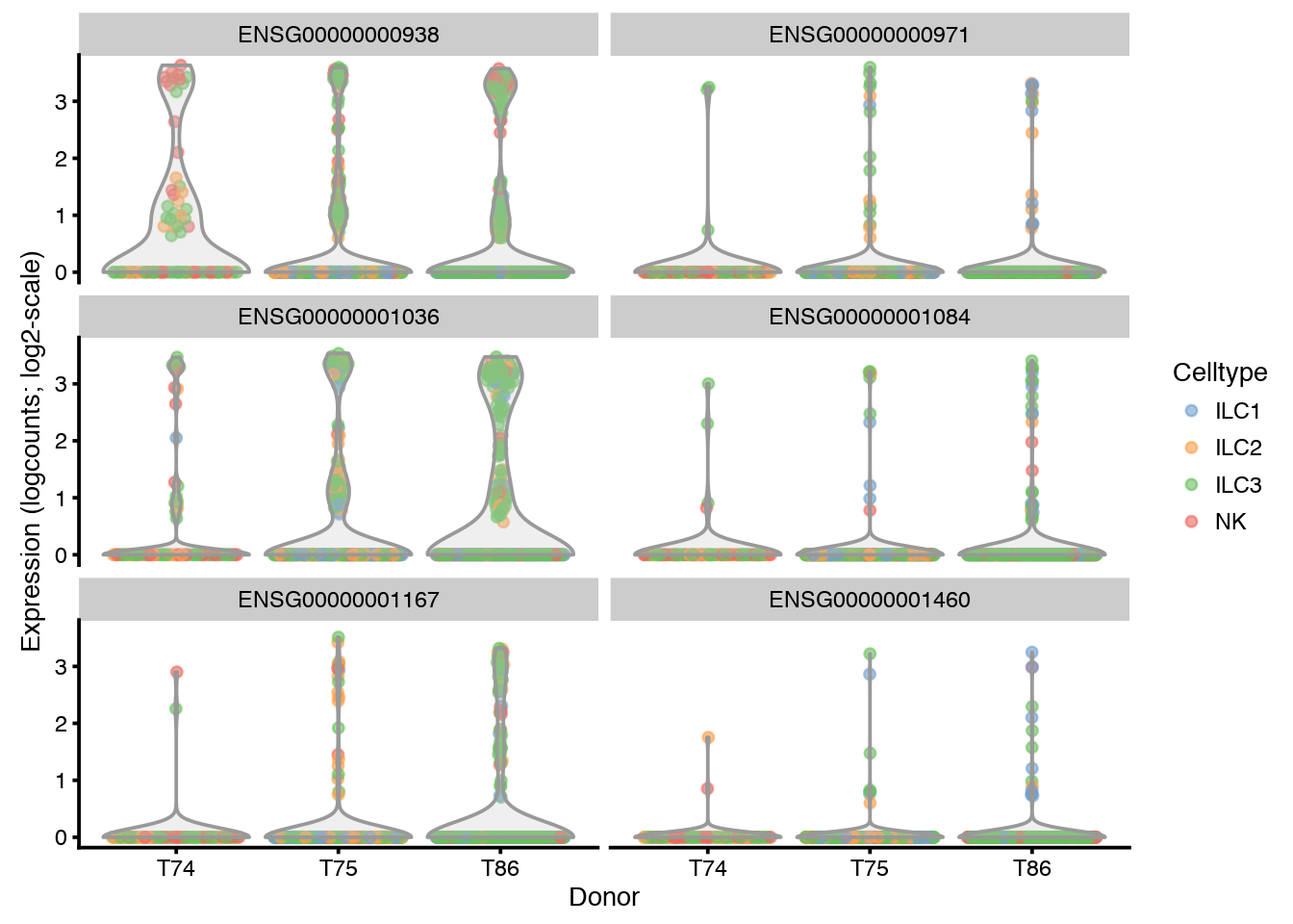

Expression can also be displayed without the violins and using different data for instance by raw counts instead. Also different grouping by Celltype instead of Donor.

plotExpression(sce, rownames(sce)[6:11],
               x = "Celltype", exprs_values = "counts", colour = "Donor",
               show_median = TRUE, show_violin = FALSE,  log = TRUE)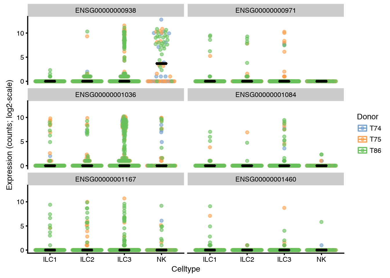

In principle you can show a lot of different data in the same plot, using:

• color_by - color cells
• shape_by - a variety of shapes
• size by - size of the cells

plotExpression(sce, rownames(sce)[6:11],
    colour_by = "Donor", shape_by = "Celltype", 
    size_by = "total_features",               
    exprs_values = "logcounts",  log=TRUE)

You can play around with all the arguments in plotExpression, for example:

• log=TRUE/FALSE
• show_violin=TRUE/FALSE
• show_median=TRUE/FALSE
• exprs_values=“counts”/“logcounts”/“fpkms” etc.

And visualization of different features onto the violoins with:

• x
• color_by
• shape_by
• size_by

6 QC overview

There are several ways to plot QC information for the cells in the scater package. A few examples are provided below. In this case, cells have already been filtered to remove low quality samples, so no filtering step is performed.

# first remove all features with no/low expression, here set to expression in more than 5 cells with > 1 count
keep_feature <- rowSums(counts(sce) > 1) > 5
sce <- sce[keep_feature,]

## Plot highest expressed genes.
plotQC(sce, type = "highest-expression",col_by="Celltype")

Plot frequency of expression (number of cells with detection) vs mean normalised expression.

plotExprsFreqVsMean(sce)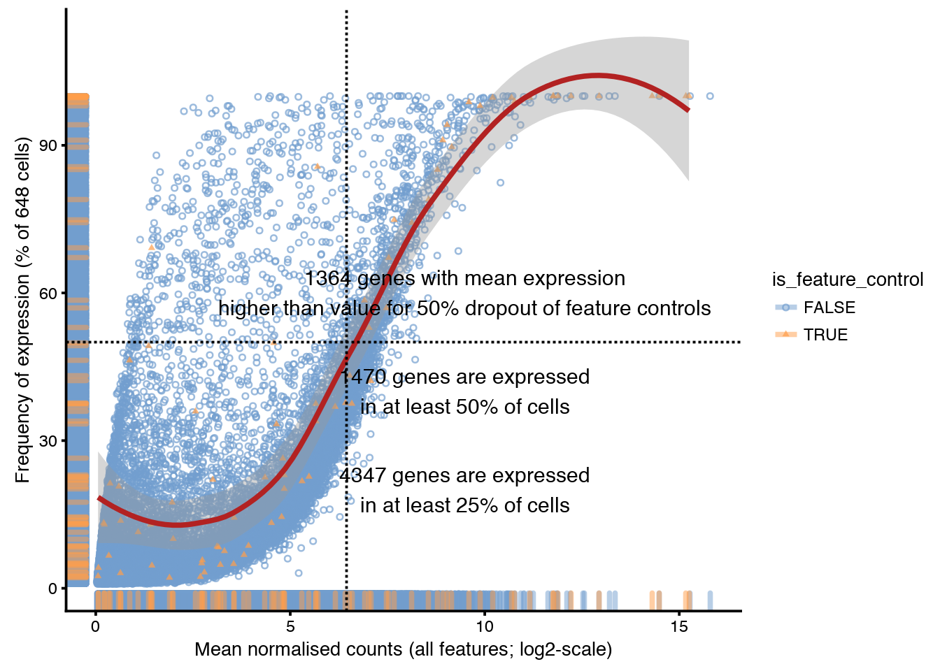

With the function plotRowData you can plot the different columns with gene information in rowData. For instance, log10 total count vs number of cells a gene is detected in. Colored by “is_feature_control” to highlight the spike-ins.

plotRowData(sce, aes_string(x = "n_cells_counts", 
                            y ="log10_total_counts",col="is_feature_control"))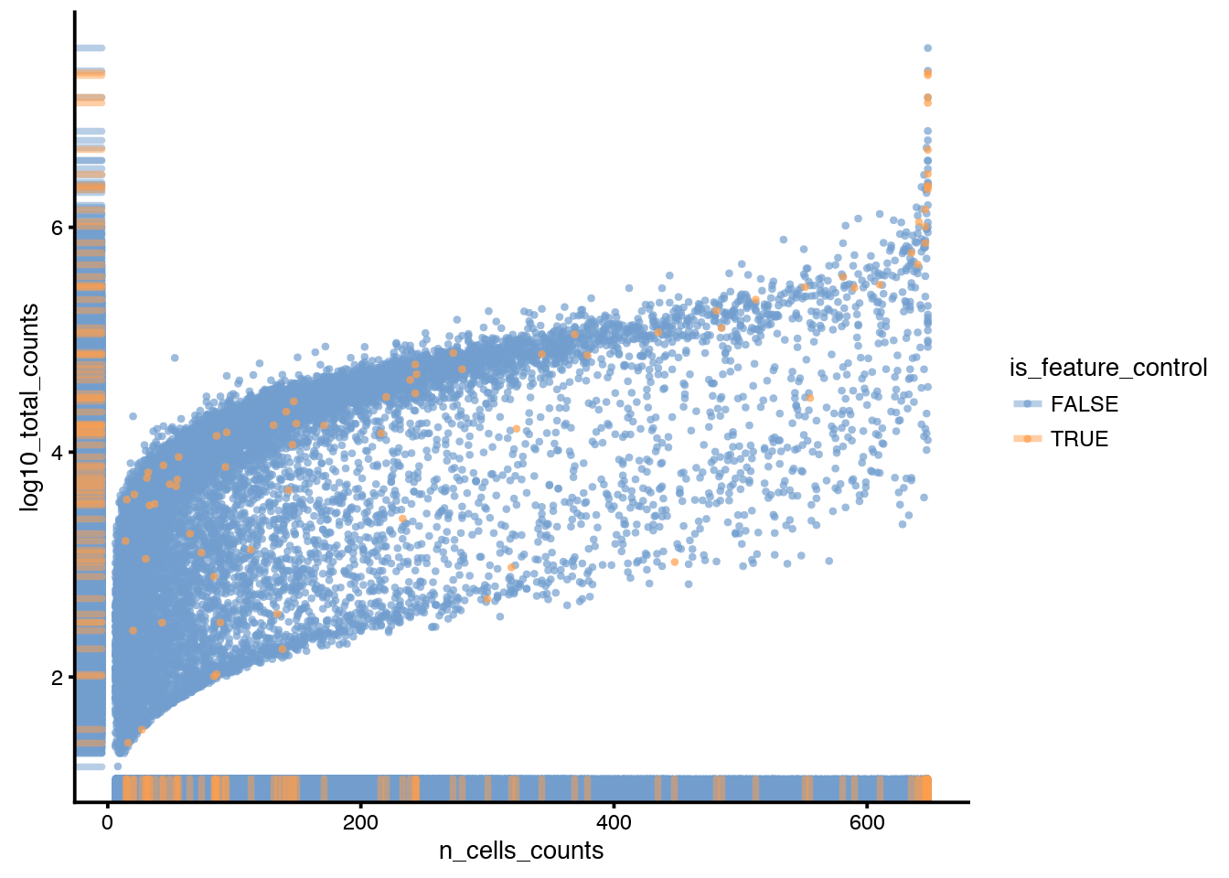

Likewise for plotColData you can plot all the columns with different cell information.

plotColData(sce, aes_string(x="total_features", 
                            y="pct_counts_ERCC", col="Donor"))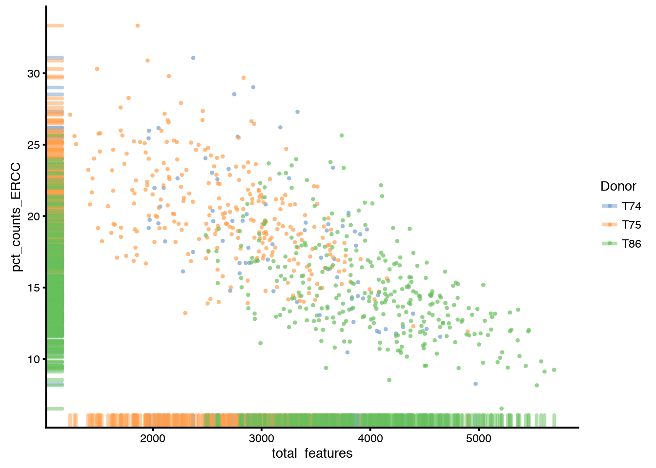

If we instead have an x-variable that is a factor, the data will be shown as a violin plot, for instance, by celltype:

plotColData(sce, aes_string(x="Celltype", 
                            y="pct_counts_ERCC"))

The function plotColData is a synonym to functions plotCellData and plotPhenoData that can be used in the same way.

Here we look again at number of detected genes (total_features) for the different donors and per celltype. And combine the 2 ggplot objects into one plot with multiplot.

p1 <- plotPhenoData(sce, aes(x = Donor, y = total_features,  
                                    colour = log10_total_counts))

p2 <- plotPhenoData(sce, aes(x = Celltype, y = total_features, 
                                     colour = log10_total_counts))

multiplot(p1, p2, rows = 2)

## [1] 2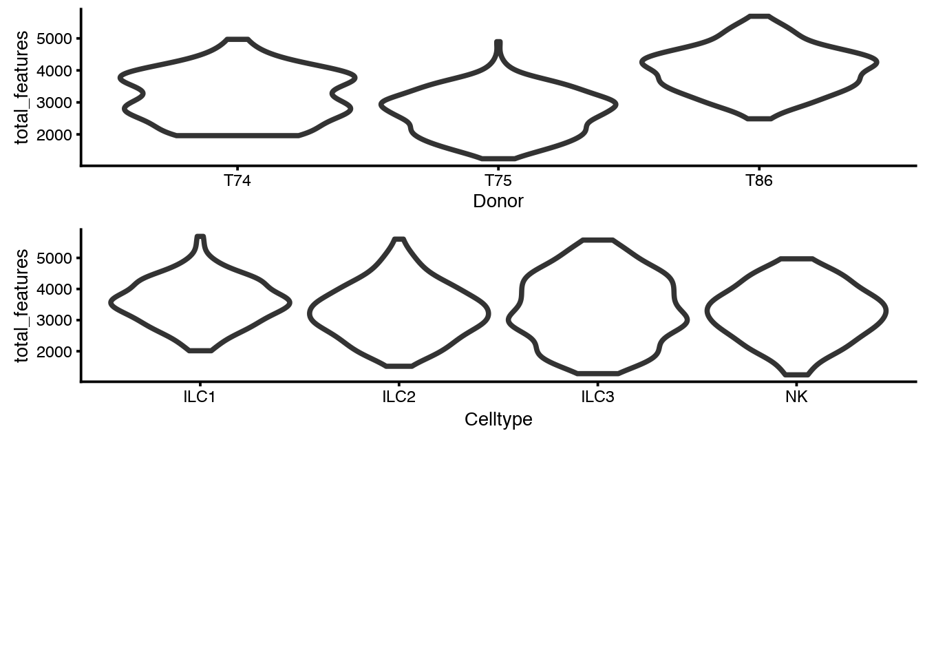

Plot the percentage of expression accounted for by feature controls against total_features.

plotPhenoData(sce, 
      aes(x = total_features, y = pct_counts_feature_control, colour = Donor)) + 
      theme(legend.position = "top") +
      stat_smooth(method = "lm", se = FALSE, size = 2, fullrange = TRUE)

7 Dimensionality reduction plots

We can plot the cells in reduced space and define color/shape/size by different qc-metrics or meta-data entries.

The function plotPCA will run PCA, but to avoid having to rerun the prcomp step, it is better to run it once with runPCA and the cell embeddings are stored in the slot sce@reducedDims$PCA.

The default is to run on top 500 variable genes (selected based on highest variance).

# run pca with top 1000 genes:
sce <- runPCA(sce, ntop = 1000, ncomponents = 10)

# PCA - with different coloring, showing first 4 components
# first by Donor
plotPCA(sce,ncomponents=4,colour_by="Celltype",shape_by="Donor")

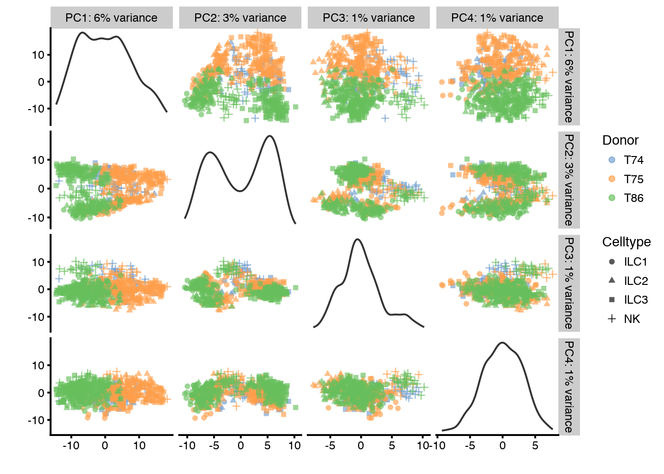
# then by Celltype
plotPCA(sce,ncomponents=4,colour_by="Donor",shape_by="Celltype")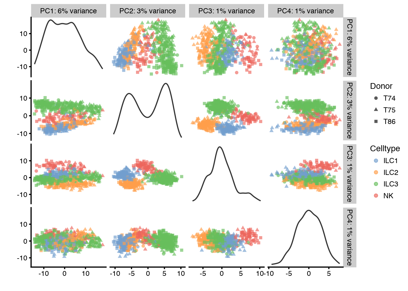

The scater package also has functions for other dimensionality reduction methods such as DiffusionMap and tSNE.

For these methods it is recommendet to include a numeric for set.seed to be able to reproduce the exact same plots.

# Diffusion map 
sce <- runDiffusionMap(sce, ncomponents = 4, rand_seed = 1)
plotDiffusionMap(sce, colour_by="Celltype",shape_by="Donor",ncomponents=4)

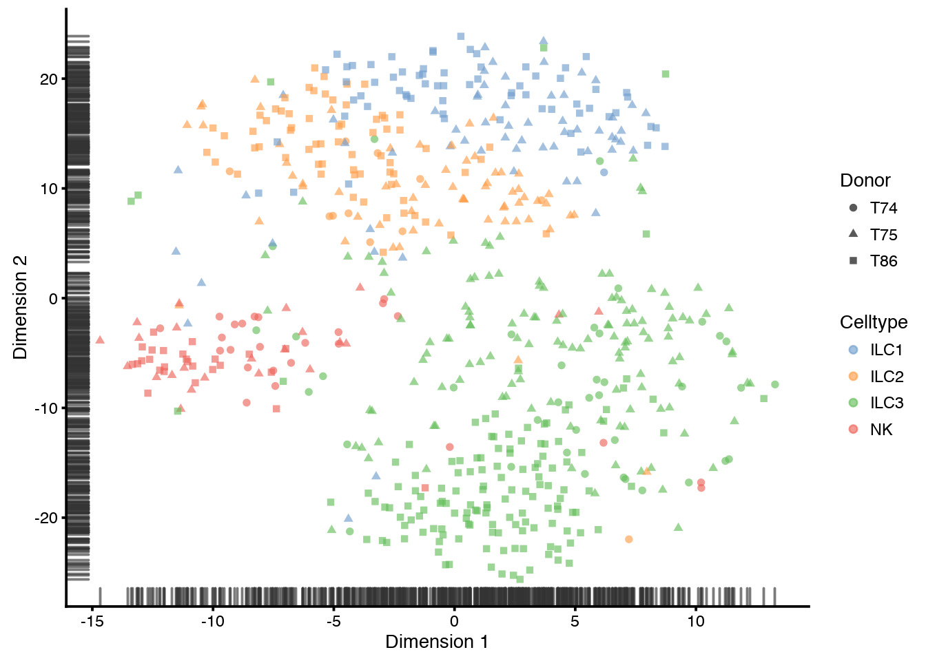
# tSNE - uses Rtsne function to run tsne, here with first 30 
sce <- runTSNE(sce,ntop=30, perplexity=30,  rand_seed = 1)

plotTSNE(sce, colour_by="Celltype",shape_by="Donor")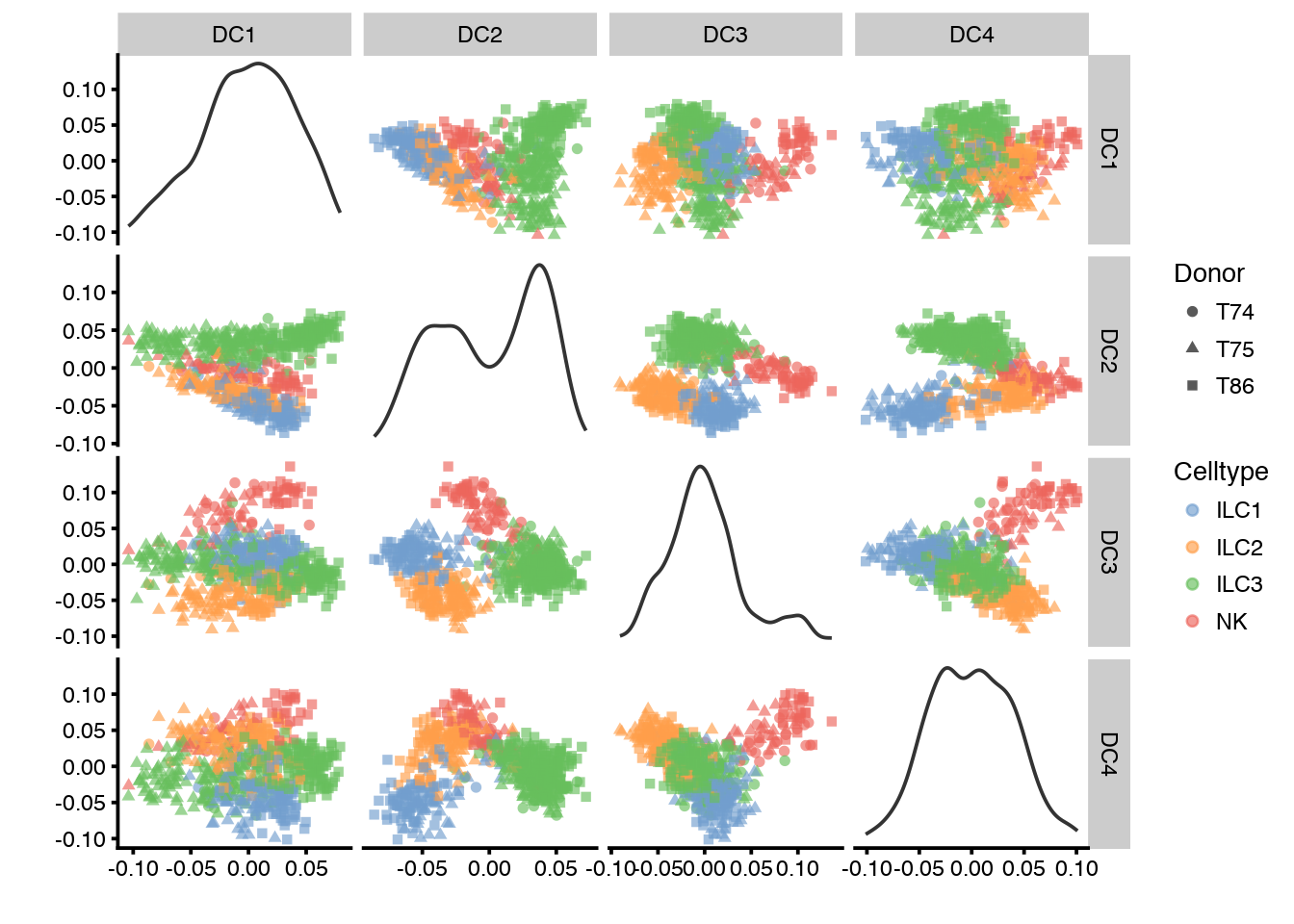

You can later plot all the reduced dimension with plotReducedDim, and select wich type with use_dimred="PCA", use_dimred="DiffusionMap" or use_dimred="TSNE" .

8 PCA based on QC-metrics

PCA based on the phenoData can be used to detect outlier cells with qc-measures that deviates from the rest. But be careful with checking how these cells deviate before taking a decision on why to remove them.

In this example dataset, no cells are assigned as outlier, hence the filtered_sce will be identical to the first sce object.

QC_sce <- runPCA(sce, pca_data_input = "pdata", 
                          detect_outliers = TRUE)

plotReducedDim(QC_sce, use_dimred="PCA", colour_by = "outlier")

# we can use the filter function to remove all outlier cells
filtered_sce <- filter(QC_sce, outlier==FALSE)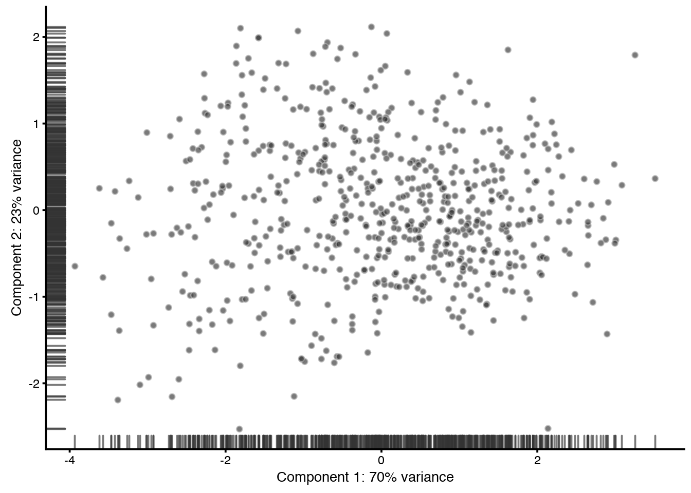

9 QC of experimental variables

Median marginal R^2 for each variable in pData(sce) when fitting a linear model regressing expression values for all genes against just that variable. Shows how much of the gene expression variation is explained by a single variable.

plotQC(sce, type = "expl")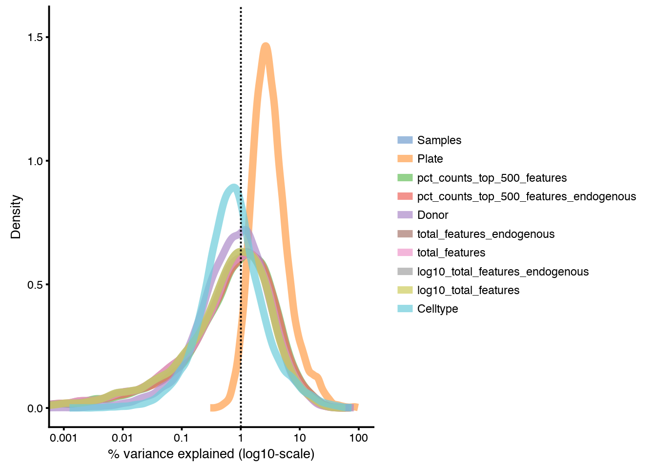

As you can see, the “Plate” variable is strongly correlating with the gene variation. This is to be expected in this dataset since distinct celltypes are sorted on different plates, but it also has more contribution than the “Celltype” variable, as we also seem to have a strong Donor batch effect.

10 QC based on PCA

Identify PCs that correlate strongly to certain QC or Meta-data values.

# for total_features
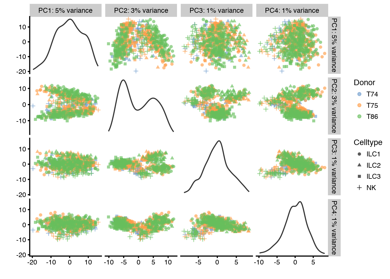
plotQC(sce, type = "find-pcs", variable = "total_features", plot_type = "pairs-pcs")

# for Donor
plotQC(sce, type = "find-pcs", variable = "Donor", plot_type = "pairs-pcs")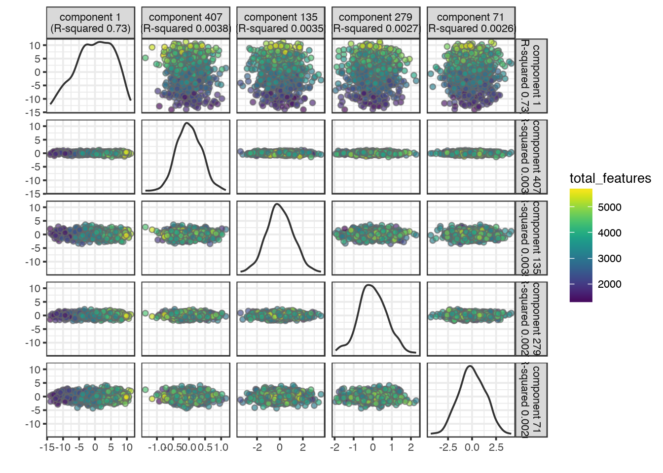

PC1 clearly correlates to total_features, which is a common problem in scRNAseq data. This may be a technical artifact, or a biological features of celltypes with very different sizes.

It is also clear that PC1 separates out the different donors.

11 Batch effect correction.

As we have discovered that we have a strong batch effect due to the diffent Donors we can adjust for that. Here we will use comBat in th SVA package for batch correction.

We also have a strong batch effect by Plate, but since there is a confounded design where some celltypes are only sorted on one plate using the Plate variable to correct for batch effect may also remove some of the biological variation.

suppressMessages(library(sva))

# remove spike-ins from matrix
C <- C[!grepl("ERCC_",rownames(C)),]

# first clean the counts table to remove non-expressed, lowly expressed genes
nExpr <- rowSums(C>1)
hist(nExpr,n=100, main="Number of cells expressed, per gene")

# as you can see, most genes are not expressed or only expressed in one cell. Remove those
C.filt <- C[nExpr>1,]

# fist construct the model matrix
mod_combat = model.matrix(~as.factor(as.character(M$Celltype)), data=M)

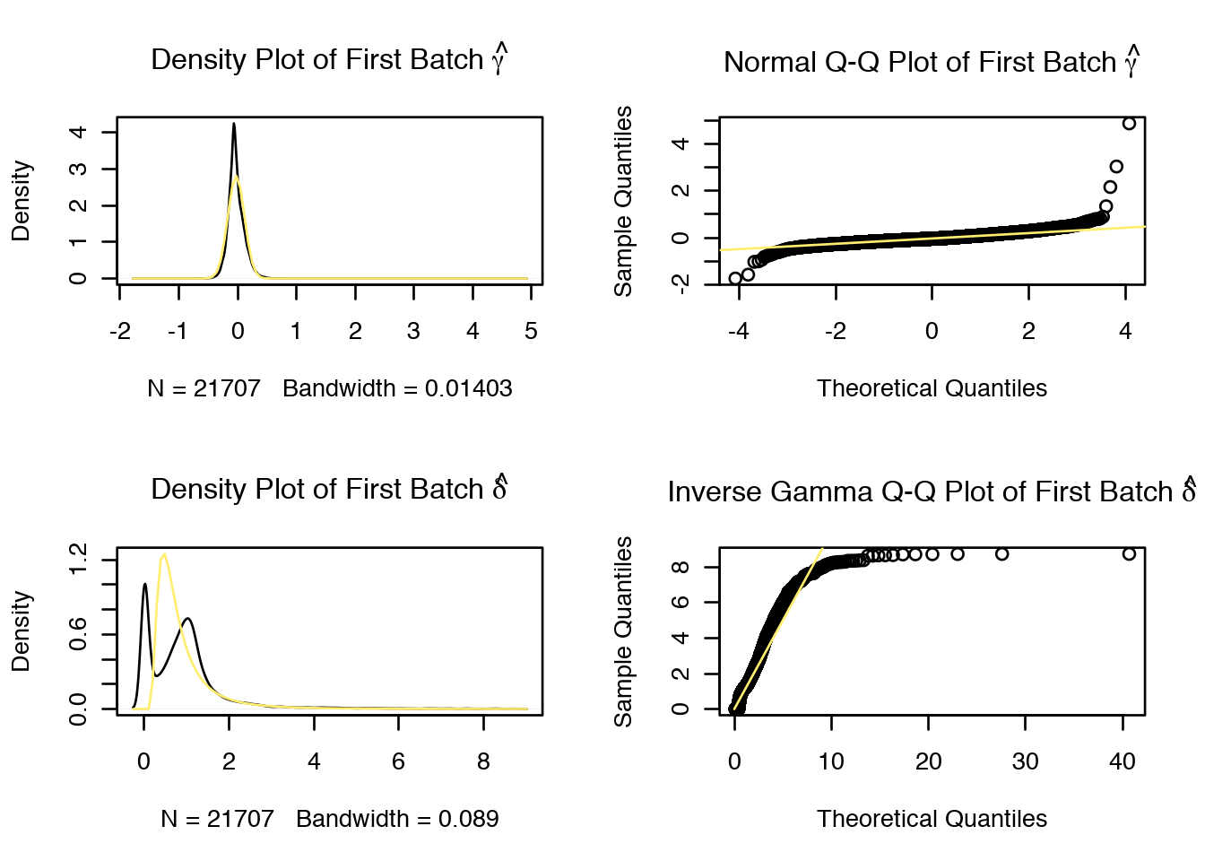
combat_ldata = ComBat(dat=as.matrix(log2(C.filt+1)), batch=M$Donor, 
                      mod=mod_combat, par.prior=TRUE, prior.plots=TRUE)

## Standardizing Data across genes

12 Scater after batch correction

Now lets create a new scater object with the corrected expression values and check the QC-stats again.

sce_combat <- SingleCellExperiment(assays = list(logcounts = as.matrix(combat_ldata)), colData = M)

# Find PCs correlated to donor
plotQC(sce_combat, type = "find-pcs", variable = "Donor", plot_type = "pairs-pcs")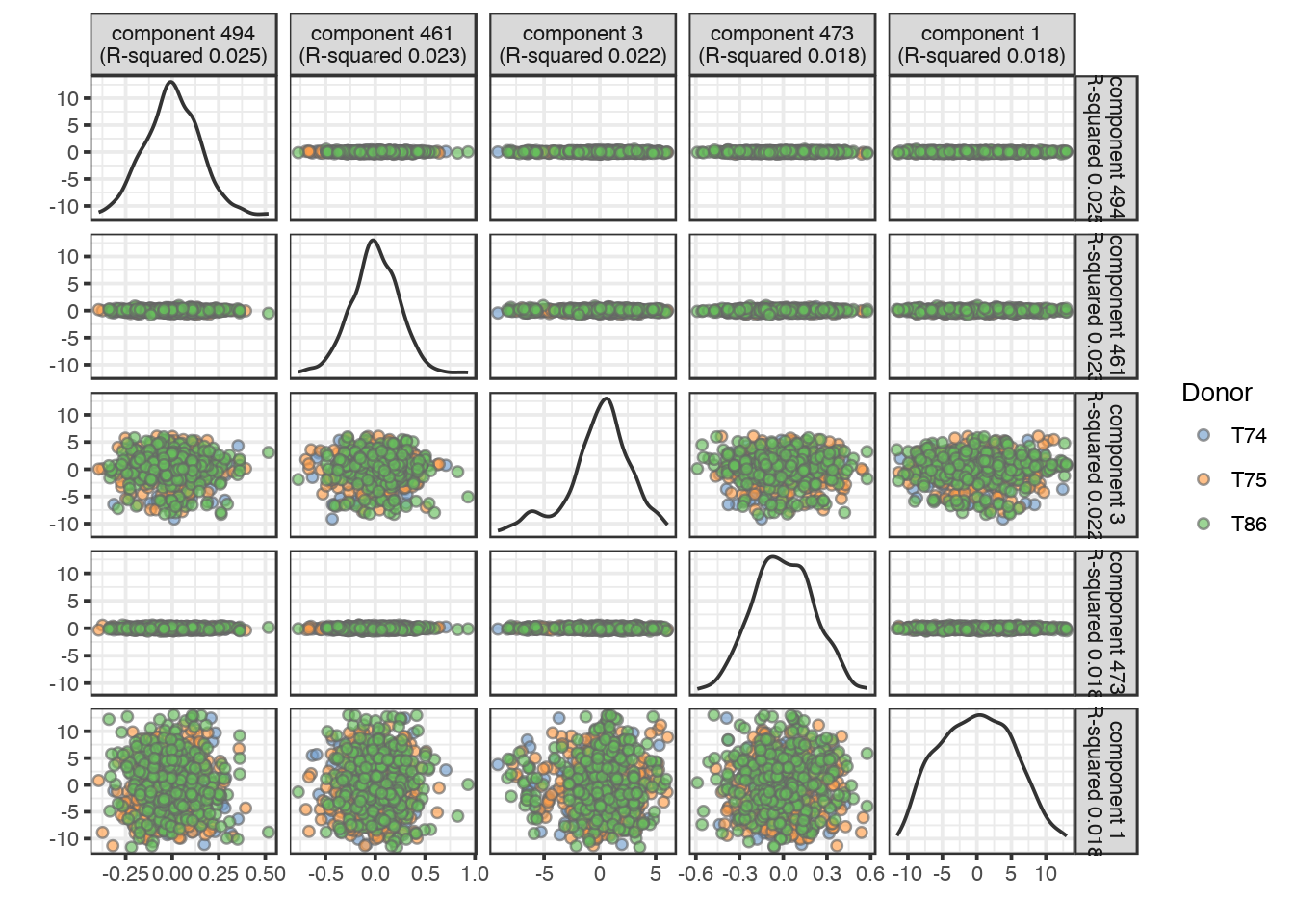

As you can see, the corrected data has no clear correlation to any of the PCs.

Plot again the same PCA as before, colored by Donor and Celltype.

# run pca with top 1000 genes:
sce_combat <- runPCA(sce_combat, ntop = 1000, ncomponents = 10)

# PCA - with different coloring, showing first 4 components
# first by Donor
plotPCA(sce_combat,ncomponents=4,colour_by="Celltype",shape_by="Donor")
# then by Celltype
plotPCA(sce_combat,ncomponents=4,colour_by="Donor",shape_by="Celltype")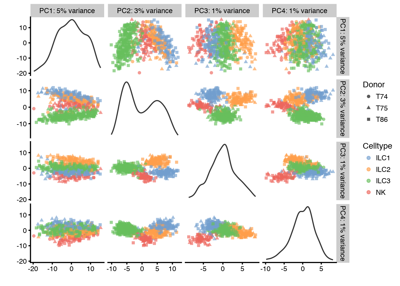

13 Save the data

As the corrected data looks better, we will use that for running SC3 in the next exercise. Save the corrected data to a file.

save(combat_ldata, file = "data/ILC/logcounts_combat_corrected.Rdata")

End of document.

14 Session Info

• This document has been created in RStudio using R Markdown and related packages.
• For R Markdown, see http://rmarkdown.rstudio.com
• For details about the OS, packages and versions, see detailed information below:

sessionInfo()

## R version 3.4.1 (2017-06-30)
## Platform: x86_64-apple-darwin15.6.0 (64-bit)
## Running under: macOS Sierra 10.12.6
## 
## Matrix products: default
## BLAS: /Library/Frameworks/R.framework/Versions/3.4/Resources/lib/libRblas.0.dylib
## LAPACK: /Library/Frameworks/R.framework/Versions/3.4/Resources/lib/libRlapack.dylib
## 
## locale:
## [1] en_US.UTF-8/en_US.UTF-8/en_US.UTF-8/C/en_US.UTF-8/en_US.UTF-8
## 
## attached base packages:
## [1] stats4    parallel  stats     graphics  grDevices utils     datasets 
## [8] methods   base     
## 
## other attached packages:
##  [1] sva_3.26.0                 BiocParallel_1.12.0       
##  [3] genefilter_1.60.0          mgcv_1.8-23               
##  [5] nlme_3.1-131               bindrcpp_0.2              
##  [7] scater_1.6.2               SingleCellExperiment_1.0.0
##  [9] SummarizedExperiment_1.8.1 DelayedArray_0.4.1        
## [11] matrixStats_0.53.0         GenomicRanges_1.30.1      
## [13] GenomeInfoDb_1.14.0        IRanges_2.12.0            
## [15] S4Vectors_0.16.0           Biobase_2.38.0            
## [17] BiocGenerics_0.24.0        forcats_0.3.0             
## [19] stringr_1.2.0              dplyr_0.7.4               
## [21] purrr_0.2.4                readr_1.1.1               
## [23] tidyr_0.8.0                tibble_1.4.2              
## [25] ggplot2_2.2.1              tidyverse_1.2.1           
## [27] captioner_2.2.3            bookdown_0.7              
## [29] knitr_1.19                
## 
## loaded via a namespace (and not attached):
##   [1] shinydashboard_0.6.1   lme4_1.1-15            RSQLite_2.0           
##   [4] AnnotationDbi_1.40.0   htmlwidgets_1.0        trimcluster_0.1-2     
##   [7] grid_3.4.1             Rtsne_0.13             munsell_0.4.3         
##  [10] destiny_2.6.1          sROC_0.1-2             colorspace_1.3-2      
##  [13] rstudioapi_0.7         robustbase_0.92-8      vcd_1.4-4             
##  [16] VIM_4.7.0              TTR_0.23-3             labeling_0.3          
##  [19] tximport_1.6.0         cvTools_0.3.2          GenomeInfoDbData_1.0.0
##  [22] mnormt_1.5-5           bit64_0.9-7            rhdf5_2.22.0          
##  [25] rprojroot_1.3-2        xfun_0.1               diptest_0.75-7        
##  [28] R6_2.2.2               ggbeeswarm_0.6.0       robCompositions_2.0.6 
##  [31] RcppEigen_0.3.3.3.1    locfit_1.5-9.1         flexmix_2.3-14        
##  [34] mvoutlier_2.0.8        bitops_1.0-6           reshape_0.8.7         
##  [37] assertthat_0.2.0       promises_1.0.1         scales_0.5.0          
##  [40] nnet_7.3-12            beeswarm_0.2.3         gtable_0.2.0          
##  [43] Cairo_1.5-9            rlang_0.2.0            MatrixModels_0.4-1    
##  [46] splines_3.4.1          lazyeval_0.2.1         acepack_1.4.1         
##  [49] broom_0.4.3            checkmate_1.8.5        yaml_2.1.16           
##  [52] reshape2_1.4.3         modelr_0.1.2           backports_1.1.2       
##  [55] httpuv_1.4.3           Hmisc_4.1-1            tools_3.4.1           
##  [58] psych_1.7.8            RColorBrewer_1.1-2     proxy_0.4-21          
##  [61] Rcpp_0.12.15           plyr_1.8.4             base64enc_0.1-3       
##  [64] progress_1.1.2         zlibbioc_1.24.0        RCurl_1.95-4.10       
##  [67] prettyunits_1.0.2      rpart_4.1-12           viridis_0.5.0         
##  [70] cowplot_0.9.2          zoo_1.8-1              haven_1.1.1           
##  [73] cluster_2.0.6          magrittr_1.5           data.table_1.10.4-3   
##  [76] SparseM_1.77           lmtest_0.9-35          mvtnorm_1.0-7         
##  [79] hms_0.4.2              mime_0.5               evaluate_0.10.1       
##  [82] xtable_1.8-2           smoother_1.1           pbkrtest_0.4-7        
##  [85] XML_3.98-1.9           mclust_5.4             readxl_1.1.0          
##  [88] gridExtra_2.3          compiler_3.4.1         biomaRt_2.34.2        
##  [91] crayon_1.3.4           minqa_1.2.4            htmltools_0.3.6       
##  [94] pcaPP_1.9-73           later_0.7.2            Formula_1.2-2         
##  [97] rrcov_1.4-3            lubridate_1.7.1        DBI_0.7               
## [100] fpc_2.1-11             MASS_7.3-48            boot_1.3-20           
## [103] Matrix_1.2-12          car_2.1-6              cli_1.0.0             
## [106] sgeostat_1.0-27        bindr_0.1              igraph_1.1.2          
## [109] pkgconfig_2.0.1        foreign_0.8-69         laeken_0.4.6          
## [112] sp_1.2-7               xml2_1.2.0             annotate_1.56.1       
## [115] vipor_0.4.5            XVector_0.18.0         rvest_0.3.2           
## [118] digest_0.6.15          pls_2.6-0              rmarkdown_1.8         
## [121] cellranger_1.1.0       htmlTable_1.11.2       edgeR_3.20.8          
## [124] kernlab_0.9-25         curl_3.1               modeltools_0.2-21     
## [127] shiny_1.1.0            quantreg_5.34          rjson_0.2.15          
## [130] nloptr_1.0.4           jsonlite_1.5           viridisLite_0.3.0     
## [133] limma_3.34.8           pillar_1.1.0           lattice_0.20-35       
## [136] GGally_1.3.2           httr_1.3.1             DEoptimR_1.0-8        
## [139] survival_2.41-3        glue_1.2.0             xts_0.10-1            
## [142] prabclus_2.2-6         bit_1.1-12             class_7.3-14          
## [145] stringi_1.1.6          blob_1.1.0             latticeExtra_0.6-28   
## [148] memoise_1.1.0          e1071_1.6-8

Page built on: 20-Jun-2018 at 11:27:42.