scRNA-Seq Analysis
Hands-On | SC3
Åsa Björklund
11-Jun-2018
![]()
Consensus clustering single-cell RNA-Seq data using the R package SC3.
Clustering of data using SC3 package. For more information on the method, please read their paper.
Their tutorial can be found at: here.
Here we run through steps 1-5 of the tutorial, part 6 is more detail on the different steps of SC3, go through that as well if you find time.
For this exercise you can either run with your own data or with the example data from Treutlein paper that they provide with the package. Below is an example with human innate lympoid cells (ILCs) from Bjorklund et al. 2016.
If you want to run the package with the ILCs, all data, plus some intermediate files for steps that takes long time, can be found in the course uppmax folder with subfolder:
data/ILC/
1 Prepare data
1.1 Load packages
suppressMessages(library(scater))
suppressMessages(library(SC3))
1.2 Read data
# read in meta data table and create pheno data
M <- read.table("data/ILC/Metadata_ILC.csv", sep=",",header=T)

# in the scater exercise, you should have created a batch corrected matrix with combat, load that one as well.
load("data/ILC/logcounts_combat_corrected.Rdata")
In this case it may be wise to translate ensembl IDs to gene names to make plots with genes more understandable. We have a file with all gene name translations.
TR <- read.table("data/ILC/gene_name_translation_biotype.tab",sep="\t")

# find the correct entries in TR and merge ensembl name and gene id.
m <- match(rownames(combat_ldata),TR$ensembl_gene_id)
newnames <- apply(cbind(as.vector(TR$external_gene_name)[m],rownames(combat_ldata)),1,paste,collapse=":")
rownames(combat_ldata)<-newnames
2 Create SCE object
Create a scater SingleCellExperiment object.
# create the SingleCellExperiement (SCE) object
sce <- SingleCellExperiment(assays =
                    list(logcounts = as.matrix(combat_ldata)), colData = M)

# To be used by SC3, the SCE object must contain "feature_symbol"
# define feature names in feature_symbol column
rowData(sce)$feature_symbol <- rownames(sce)
In this example we fill all slots, fpkm, counts and logcounts, to show how it can be done. However, for running SC3 it is only necessary to have the logcounts slot, since that is what is used.
2.1 QC with scater
Use scater package to calculate qc-metrics and plot a PCA
sce <- calculateQCMetrics(sce, exprs_values ="logcounts")
sce <- runPCA(sce, ntop = 1000)
plotPCA(sce, colour_by = "Celltype",
        exprs_values = "logcounts", shape_by = "Donor")

plotPCA(sce, colour_by = "Donor",
        exprs_values = "logcounts", shape_by = "Celltype")

3 Run SC3
OBS! It takes a while to run (~30 mins for this data set size and a single core), define number of clusters to test with ks parameter, testing more different k’s will take longer time. You can get a hint on number of clusters you should set by running the sc3_estimate_k function, but it may not always give the biologically relevant clusters.
In this case we will only test with 2 different k’s, 4 & 6 for speed. But it is recommended to run a wider range.
# since this step takes a while, save data to a file so that it does not have to be rerun if you execute the code again.
# A precomputed file is available in the data/ILC/ folder

savefile <- "data/ILC/sc3_combatdata_ilc_k4.6.Rdata"
if (file.exists(savefile)){
   load(savefile)
}else {
   sce <- sc3(sce, ks = c(4,6), biology = TRUE, gene_filter = FALSE, n_cores = 1)
   save(sce,file=savefile)
}
4 Shiny app.
Now you can explore the data interactively within a shiny app using command:
sc3_interactive(sce)
5 Plot results
Instead of using the app, that sometimes is very slow, you can also create each plot with different commands, below are some example plots.
All clustering info should be stored in the colData slot of the SCE object.
colnames(colData(sce))## [1] "Samples" "Plate"
## [3] "Donor" "Celltype"
## [5] "total_features" "log10_total_features"
## [7] "total_logcounts" "log10_total_logcounts"
## [9] "pct_logcounts_top_50_features" "pct_logcounts_top_100_features"
## [11] "pct_logcounts_top_200_features" "pct_logcounts_top_500_features"
## [13] "is_cell_control" "sc3_4_clusters"
## [15] "sc3_6_clusters" "sc3_4_log2_outlier_score"
## [17] "sc3_6_log2_outlier_score"And in the rowData slot, there should be some annotations for the genes, with regards to marker discovery usin AUROC test or differential expression using Kruskal-Wallis test.
colnames(rowData(sce))## [1] "feature_symbol" "is_feature_control"
## [3] "mean_logcounts" "log10_mean_logcounts"
## [5] "rank_logcounts" "n_cells_logcounts"
## [7] "pct_dropout_logcounts" "sc3_gene_filter"
## [9] "sc3_4_markers_clusts" "sc3_4_markers_padj"
## [11] "sc3_4_markers_auroc" "sc3_6_markers_clusts"
## [13] "sc3_6_markers_padj" "sc3_6_markers_auroc"
## [15] "sc3_4_de_padj" "sc3_6_de_padj"5.1 Visualize
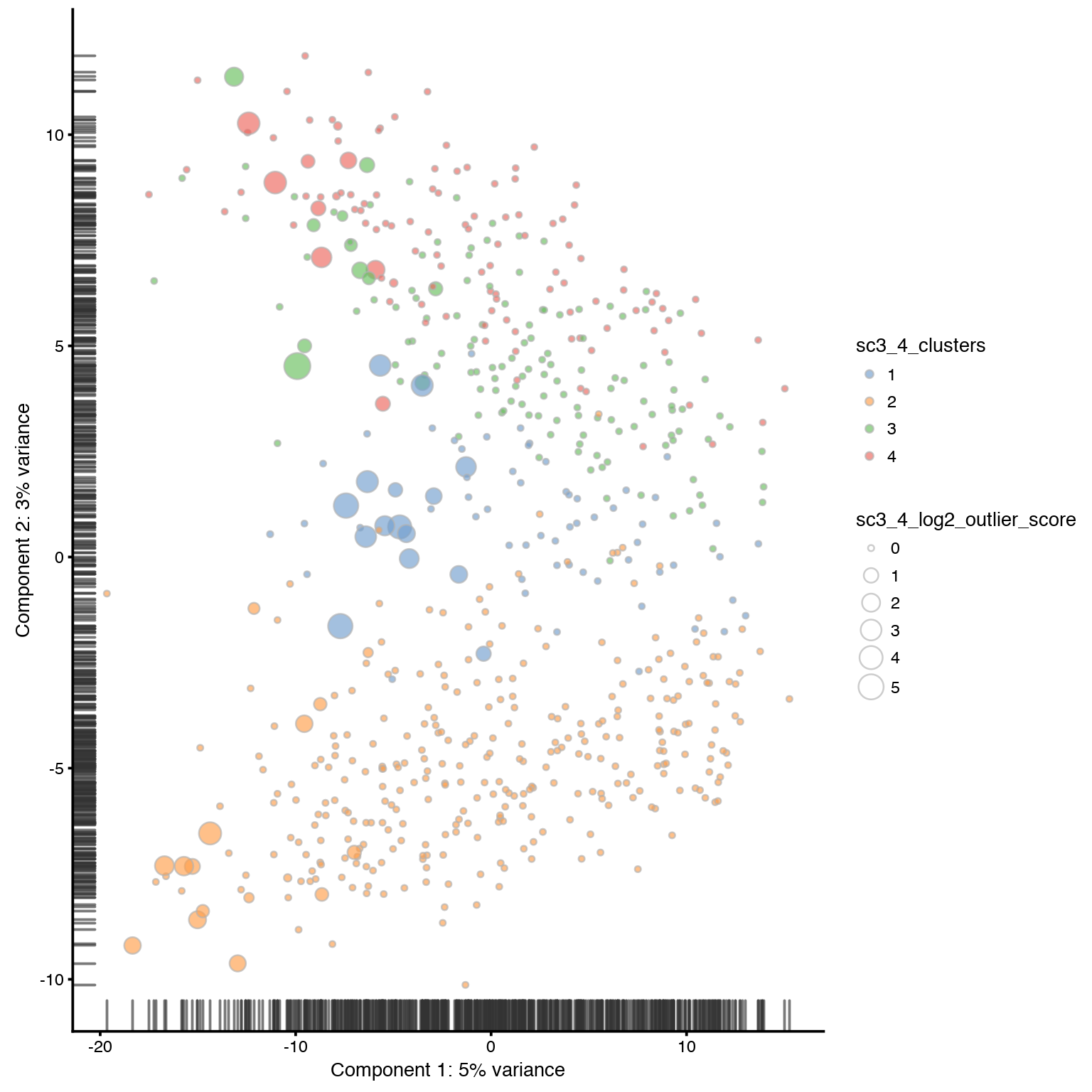
Plot SC3 clustering results onto PCA.
# plot PCA for 4 clusters
plotPCA(sce,
    colour_by = "sc3_4_clusters",
    size_by = "sc3_4_log2_outlier_score"
)
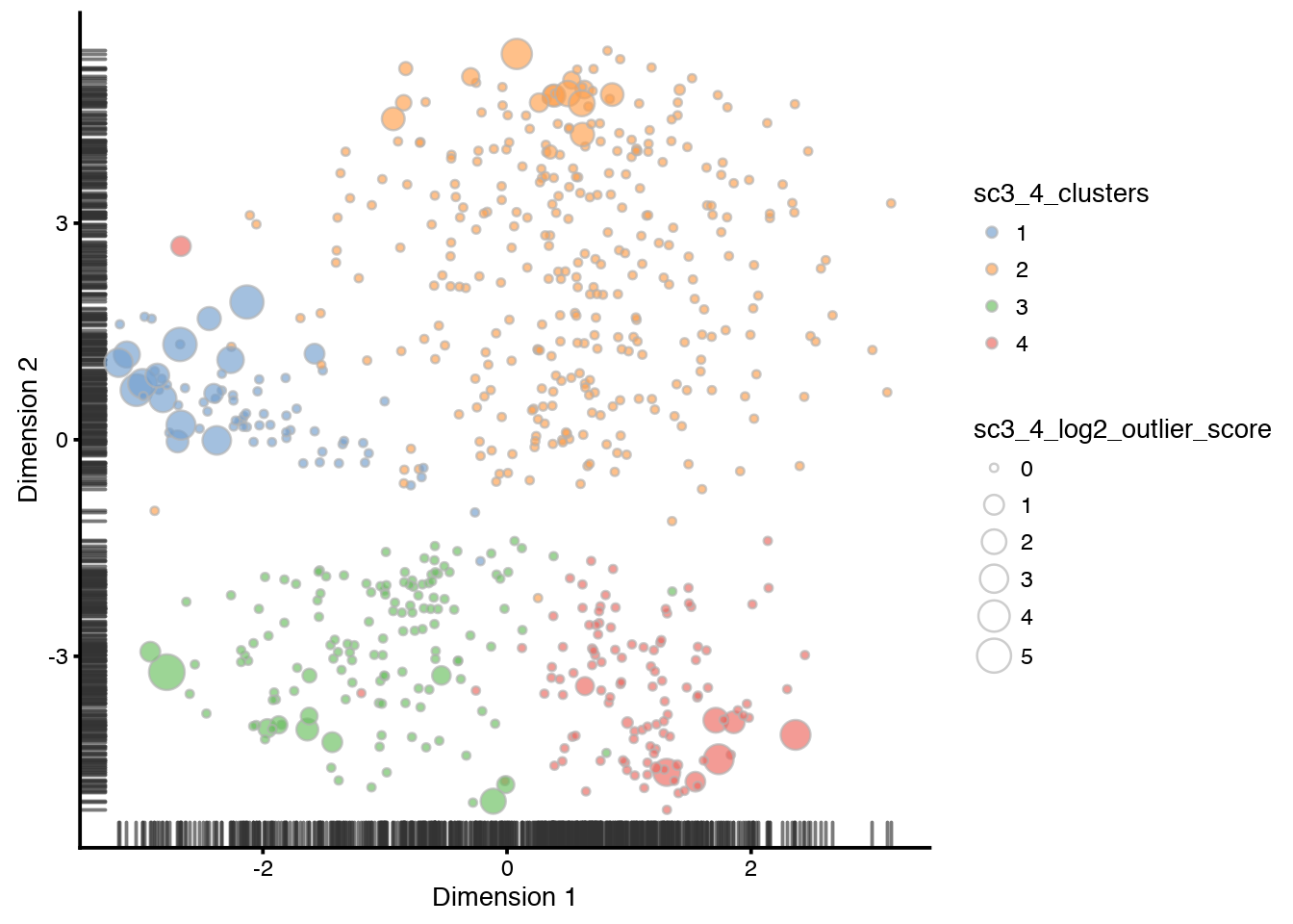
And onto the tSNE, both with k=4 and k=6.
sce <- runTSNE(sce, ntop = 100, n_dimred = 10, rand_seed = 1)
plotTSNE(sce,
colour_by = "sc3_4_clusters",
size_by = "sc3_4_log2_outlier_score"
)
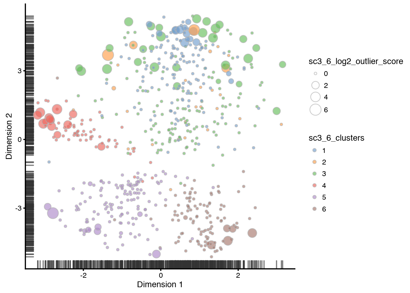
plotTSNE(sce,
colour_by = "sc3_6_clusters",
size_by = "sc3_6_log2_outlier_score"
)
5.2 Explore clusters
Plot consensus clustering with k=4, also displaying info on Celltype, Donor, detected genes, clustering and outlier scores from SC3.
sc3_plot_consensus(
    sce, k = 4,
    show_pdata = c(
        "Celltype",
        "log10_total_features",
        "sc3_4_clusters",
        "sc3_4_log2_outlier_score",
    "Donor"
    )
)
SC3 clearly groups the 4 main celltypes, but within celltypes there is clear separation of the donors, in spite of us using batch correction.
Same plot but with k=6.
# same with 6 clusters
sc3_plot_consensus(
    sce, k = 6,
    show_pdata = c(
        "Celltype",
        "log10_total_features",
        "sc3_6_clusters",
        "sc3_6_log2_outlier_score",
    "Donor"
    )
)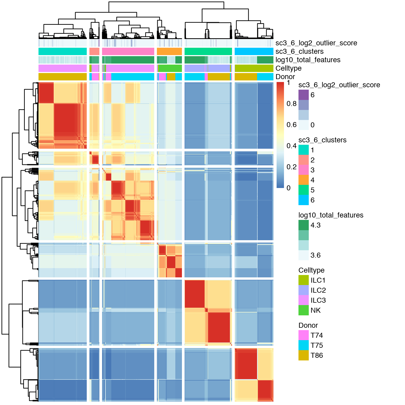
With k=6 the ILC3 population is split into 2 main clusters and one very small cluster (cluster 1 with only 2 cells), that is mainly based on donor origin.
Plot how many high auc value genes there are assigned per cluster, also color by p-value. Could give an indication of how confident we can be about each cluster split.
plotFeatureData(
    sce,
    aes(
        x = sc3_6_markers_clusts,
        y = sc3_6_markers_auroc,
        colour = sc3_6_markers_padj
    )
)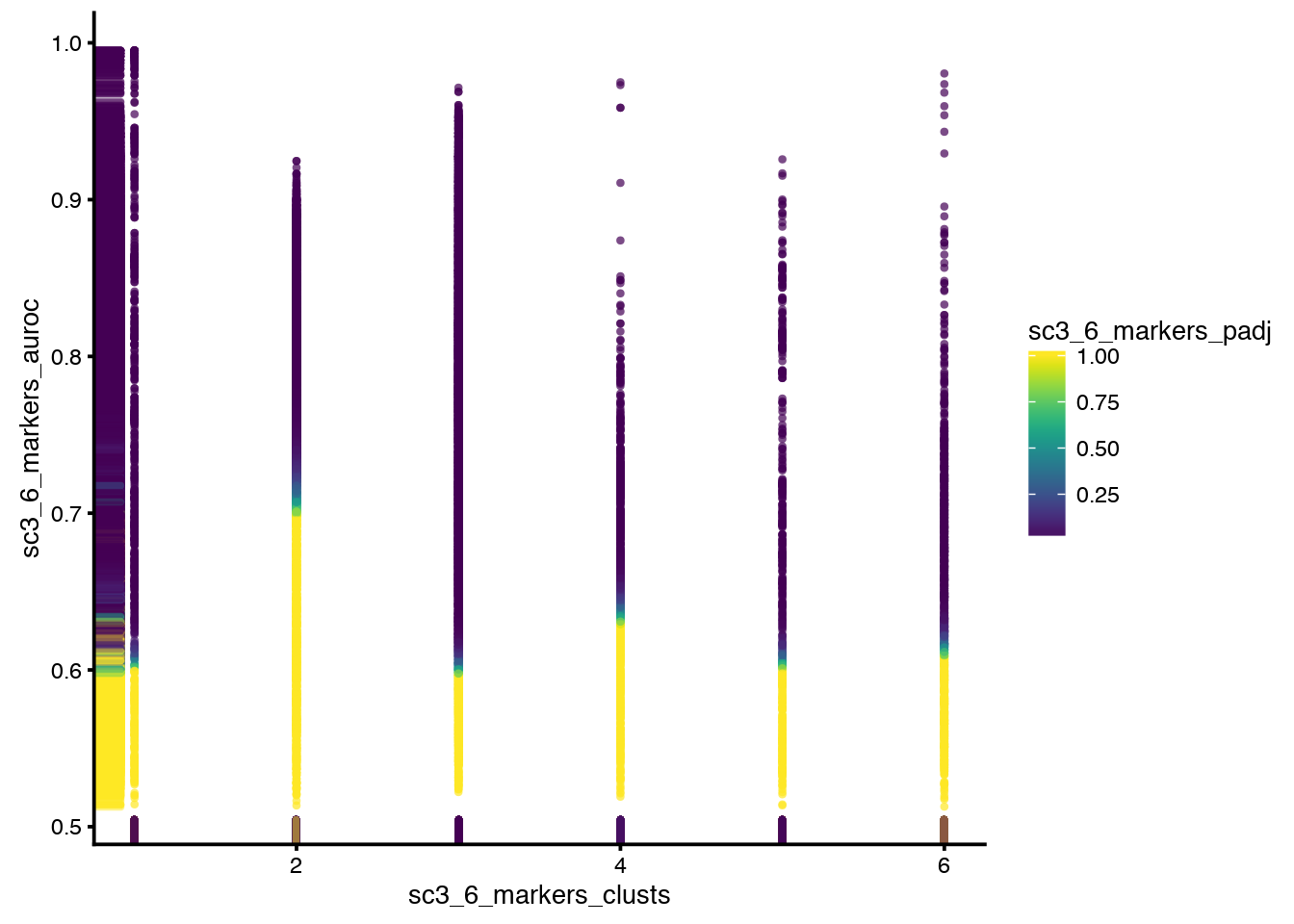
Clearly, cluster 1 has no significant genes, wich would give lower confidence in that cluster.
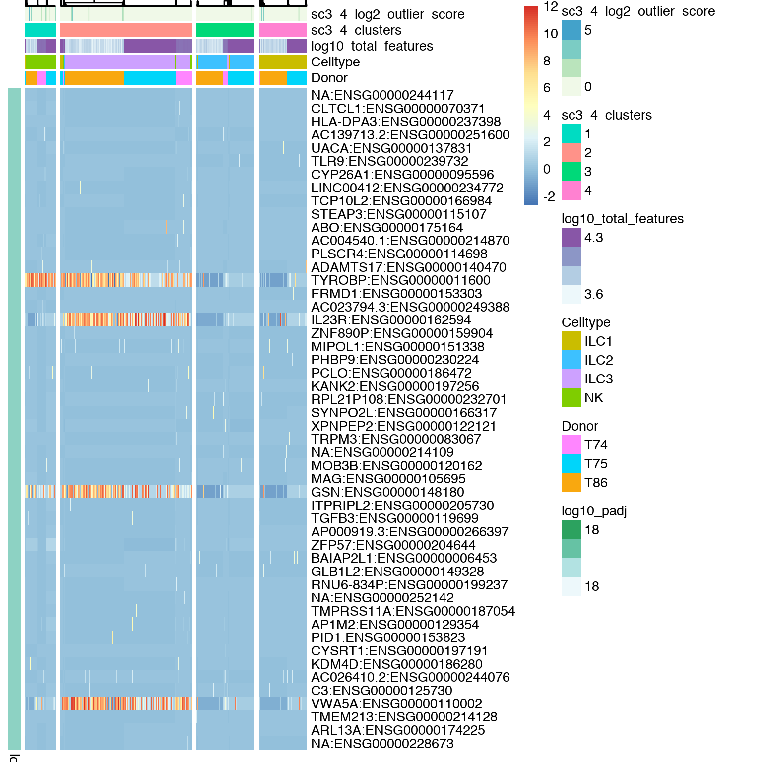
Plot marker genes for the clusters, as defined with the AUROC test. By default the genes with the area under the ROC curve (AUROC) > 0.85 and with the p-value < 0.01 are selected and the top 10 marker genes of each cluster are visualized in this heatmap.
# plot expression of gene clusters
sc3_plot_markers(sce, k = 4,
    show_pdata = c(
        "Celltype",
        "log10_total_features",
        "sc3_4_clusters",
        "sc3_4_log2_outlier_score",
    "Donor"
    )
)
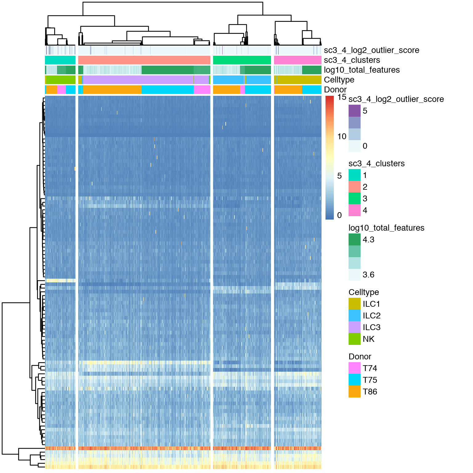
Plot clustering of all gene’s expression. This plots shows a clustering of the genes (kmeans clustering with k=100) and their joint expression in the different cell clusters.
# plot expression of gene clusters
sc3_plot_expression(sce, k = 4,
    show_pdata = c(
        "Celltype",
        "log10_total_features",
        "sc3_4_clusters",
        "sc3_4_log2_outlier_score",
    "Donor"
    )
)
DE genes, these are estimated using the non-parametric Kruskal-Wallis test.
# plot DE genes
sc3_plot_de_genes(sce, k = 4,
    show_pdata = c(
        "Celltype",
        "log10_total_features",
        "sc3_4_clusters",
        "sc3_4_log2_outlier_score",
    "Donor"
    )
)
End of document.
6 Session Info
- This document has been created in RStudio using R Markdown and related packages.
- For R Markdown, see http://rmarkdown.rstudio.com
- For details about the OS, packages and versions, see detailed information below:
sessionInfo()## R version 3.4.1 (2017-06-30)
## Platform: x86_64-apple-darwin15.6.0 (64-bit)
## Running under: macOS Sierra 10.12.6
##
## Matrix products: default
## BLAS: /Library/Frameworks/R.framework/Versions/3.4/Resources/lib/libRblas.0.dylib
## LAPACK: /Library/Frameworks/R.framework/Versions/3.4/Resources/lib/libRlapack.dylib
##
## locale:
## [1] en_US.UTF-8/en_US.UTF-8/en_US.UTF-8/C/en_US.UTF-8/en_US.UTF-8
##
## attached base packages:
## [1] stats4 parallel stats graphics grDevices utils datasets
## [8] methods base
##
## other attached packages:
## [1] SC3_1.7.7 scater_1.6.2
## [3] SingleCellExperiment_1.0.0 SummarizedExperiment_1.8.1
## [5] DelayedArray_0.4.1 matrixStats_0.53.0
## [7] GenomicRanges_1.30.1 GenomeInfoDb_1.14.0
## [9] IRanges_2.12.0 S4Vectors_0.16.0
## [11] Biobase_2.38.0 BiocGenerics_0.24.0
## [13] forcats_0.3.0 stringr_1.2.0
## [15] dplyr_0.7.4 purrr_0.2.4
## [17] readr_1.1.1 tidyr_0.8.0
## [19] tibble_1.4.2 ggplot2_2.2.1
## [21] tidyverse_1.2.1 captioner_2.2.3
## [23] bookdown_0.7 knitr_1.19
##
## loaded via a namespace (and not attached):
## [1] readxl_1.1.0 backports_1.1.2 plyr_1.8.4
## [4] lazyeval_0.2.1 shinydashboard_0.6.1 digest_0.6.15
## [7] foreach_1.4.4 htmltools_0.3.6 viridis_0.5.0
## [10] gdata_2.18.0 magrittr_1.5 memoise_1.1.0
## [13] cluster_2.0.6 doParallel_1.0.11 ROCR_1.0-7
## [16] limma_3.34.8 modelr_0.1.2 prettyunits_1.0.2
## [19] colorspace_1.3-2 blob_1.1.0 rvest_0.3.2
## [22] rrcov_1.4-3 WriteXLS_4.0.0 haven_1.1.1
## [25] xfun_0.1 crayon_1.3.4 RCurl_1.95-4.10
## [28] jsonlite_1.5 tximport_1.6.0 bindr_0.1
## [31] iterators_1.0.9 glue_1.2.0 registry_0.5
## [34] gtable_0.2.0 zlibbioc_1.24.0 XVector_0.18.0
## [37] DEoptimR_1.0-8 scales_0.5.0 pheatmap_1.0.8
## [40] mvtnorm_1.0-7 DBI_0.7 edgeR_3.20.8
## [43] rngtools_1.2.4 Rcpp_0.12.15 viridisLite_0.3.0
## [46] xtable_1.8-2 progress_1.1.2 foreign_0.8-69
## [49] bit_1.1-12 httr_1.3.1 gplots_3.0.1
## [52] RColorBrewer_1.1-2 pkgconfig_2.0.1 XML_3.98-1.9
## [55] locfit_1.5-9.1 labeling_0.3 rlang_0.2.0
## [58] reshape2_1.4.3 later_0.7.2 AnnotationDbi_1.40.0
## [61] munsell_0.4.3 cellranger_1.1.0 tools_3.4.1
## [64] cli_1.0.0 RSQLite_2.0 broom_0.4.3
## [67] evaluate_0.10.1 yaml_2.1.16 bit64_0.9-7
## [70] robustbase_0.92-8 caTools_1.17.1 bindrcpp_0.2
## [73] nlme_3.1-131 doRNG_1.6.6 mime_0.5
## [76] xml2_1.2.0 biomaRt_2.34.2 compiler_3.4.1
## [79] rstudioapi_0.7 beeswarm_0.2.3 e1071_1.6-8
## [82] pcaPP_1.9-73 stringi_1.1.6 lattice_0.20-35
## [85] Matrix_1.2-12 psych_1.7.8 pillar_1.1.0
## [88] data.table_1.10.4-3 cowplot_0.9.2 bitops_1.0-6
## [91] httpuv_1.4.3 R6_2.2.2 promises_1.0.1
## [94] KernSmooth_2.23-15 gridExtra_2.3 vipor_0.4.5
## [97] codetools_0.2-15 gtools_3.5.0 assertthat_0.2.0
## [100] rhdf5_2.22.0 pkgmaker_0.22 rprojroot_1.3-2
## [103] rjson_0.2.15 mnormt_1.5-5 GenomeInfoDbData_1.0.0
## [106] hms_0.4.2 grid_3.4.1 class_7.3-14
## [109] rmarkdown_1.8 Rtsne_0.13 Cairo_1.5-9
## [112] shiny_1.1.0 lubridate_1.7.1 ggbeeswarm_0.6.0Page built on: 11-Jun-2018 at 16:15:16.
2018 | SciLifeLab > NBIS > RaukR 
