Reproducible Research
Hands-On Excercises
Roy Francis
28-May-2018
![]()
This is the hands-on material for Reproducible Research. These are series of excercises to help you get started with reproducible research using R. The code is hidden by default. Click on the ‘Code’ button on the right side to show the code. You can consult the R Markdown cheatsheet for quick reference.
- Familiarise yourself with Markdown/R Markdown syntax and commonly used snippets.
- Set up a project in R
- Prepare an R Markdown document
- Add content and export to some common formats
1 RStudio
Create a new project in RStudio by going to File > New Project > New Directory. Select New Project if required. Then label the project name and the directory.
An empty project is created. The R session has been refreshed. All variables are removed and the environment is cleared.
Create a new R Markdown file by going to File > New File > R Markdown.... Use the default options.
2 R Markdown
Commonly used R Markdown usage.
2.1 YAML
The content on the top of the R Markdown document in three dashes is the YAML matter. The YAML matter for this document is as below:
---
title: "Reproducible Research"
subtitle: "Hands-On Excercises"
author: "Roy Francis"
date: "`r format(Sys.Date(),format='%d-%b-%Y')`"
output:
  bookdown::html_document2:
    toc: true
    toc_float: true
    toc_depth: 3
    number_sections: true
    theme: united
    highlight: tango
    df_print: paged
    code_folding: "none"
    self_contained: false
    keep_md: false
    encoding: "UTF-8"
    css: ["assets/course.css"]
---
The title, subtitle, author and date is displayed at the top of the rendered document in a pre-specified .css style. In the above example the data is automatically printed using the r function Sys.Date(). Argument output is used to specify output document type and related arguments. rmarkdown::html_document is used to specify the standard HTML output. rmarkdown::pdf_document is used to specify the standard PDF output. Sub arguments differ depending on the output document type. Above are some of the arguments that can be supplied to the HTML document type. theme is used to specify the document style such as the font and layout. highlight is used to specify the code highlighting style. toc specifies that a table of contents must be included. Use ?rmarkdown::html_document for description of all the various options.
2.2 Text
The above level 2 heading was created by specifying ## Text. Other headings can be specified similarily.
## Level 2 heading
### Level 3 heading
#### Level 4 heading
##### Level 5 heading
###### Level 6 heading
Italic text like this This is italic text can be specified using *This is italic text* or _This is italic text_. Bold text like this This is bold text can be specified using **This is italic text** or **This is italic text**. Subscript written like this H~2~O renders as H2O. Superscript written like this 2^10^ renders as 210.
Bullet points are usually specified using an asterisk (+ or -).
+ Point one
+ Point two- Point one
- Point two
Block quotes can be specified using >.
> This is a block quote. This
> paragraph has two lines.
This is a block quote. This paragraph has two lines.
Lists can also be created inside block quotes.
> 1. This is a list inside a block quote.
> 2. Second item.
- This is a list inside a block quote.
- Second item.
Links can be created using [this](https://rmarkdown.rstudio.com/) like this.
2.3 Code
Text can be formatted as code. Code is displayed using monospaced font. Code formatting that stands by itself as a paragraph is called block code. Block codes are specified using three backticks ``` followed by code and then three more backticks.
This text below
```
This is generic block code.
```
renders like this
This is generic block code.Code formatting can also be included in the middle of a sentence. This is called inline code formatting. Using this `This is an inline formatted code.` renders like this: This is an inline formatted code.
The above codes are not actually executed. They are just text formatted in a different font. Code can be executed by specifying the language along with the backticks. Block code formatted as such:
```{r}
str(iris)
```
renders like this:
str(iris)## 'data.frame': 150 obs. of 5 variables:
## $ Sepal.Length: num 5.1 4.9 4.7 4.6 5 5.4 4.6 5 4.4 4.9 ...
## $ Sepal.Width : num 3.5 3 3.2 3.1 3.6 3.9 3.4 3.4 2.9 3.1 ...
## $ Petal.Length: num 1.4 1.4 1.3 1.5 1.4 1.7 1.4 1.5 1.4 1.5 ...
## $ Petal.Width : num 0.2 0.2 0.2 0.2 0.2 0.4 0.3 0.2 0.2 0.1 ...
## $ Species : Factor w/ 3 levels "setosa","versicolor",..: 1 1 1 1 1 1 1 1 1 1 ...Code blocks are called chunks. The chunk is executed when this document is rendered. The rendered code output is also given code highlighting based on the language. For example;
This code chunk
```{r,eval=FALSE}
ggplot(dfr4,aes(x=Month,y=fraction,colour=Year,group=Year))+
  geom_point(size=2)+
  geom_line()+
  labs(x="Month",y="Fraction of support issues")+
  scale_colour_manual(values=c("#000000","#E69F00","#56B4E9",
  "#009E73","#F0E442","#006699","#D55E00","#CC79A7"))+
  theme_bw(base_size=12,base_family="Gidole")+
  theme(panel.border=element_blank(),
        panel.grid.minor=element_blank(),
        panel.grid.major.x=element_blank(),
        axis.ticks=element_blank())
```
when rendered (not evaluated) looks like
ggplot(dfr4,aes(x=Month,y=fraction,colour=Year,group=Year))+
  geom_point(size=2)+
  geom_line()+
  labs(x="Month",y="Fraction of support issues")+
  scale_colour_manual(values=c("#000000","#E69F00","#56B4E9",
  "#009E73","#F0E442","#006699","#D55E00","#CC79A7"))+
  theme_bw(base_size=12,base_family="Gidole")+
  theme(panel.border=element_blank(),
        panel.grid.minor=element_blank(),
        panel.grid.major.x=element_blank(),
        axis.ticks=element_blank())
The chunk has several options which can be used to control chunk properties.
Using `{r,eval=FALSE}` prevents that chunk from being executed. Using `{r,echo=FALSE}` prevents the code from that chunk from being displayed. Using `{r,results="hide"}` hides the output from that chunk.
| Option | Default | Description |
|---|---|---|
| eval | TRUE | Evaluates the code in this chunk |
| echo | TRUE | Display the code |
| results | “markup” | “markup”,“asis”,“hold” or “hide” |
| warning | TRUE | Display warnings from code execution |
| error | FALSE | Display error from code execution |
| message | TRUE | Display messages from this chunk |
| tidy | FALSE | Reformat code in to be tidy |
| cache | FALSE | Cache results for future renders |
| comment | “##” | Character to prefix result output |
Chunk options are specified like this:
```{r,eval=FALSE,echo=FALSE,fig.height=6,fig.width=7}
```
2.4 Images
Images can be displayed using . For example:

This is a caption
For more control over image size, raw HTML needs to be used. For example;
<img src="rr_lab_assets/summer.jpg" width="100px">
2.5 Plots
R Plots can be plotted like below:
```{r,fig.height=6,fig.width=6}
plot(x=iris$Petal.Length,y=iris$Petal.Width)
```plot(x=iris$Petal.Length,y=iris$Petal.Width)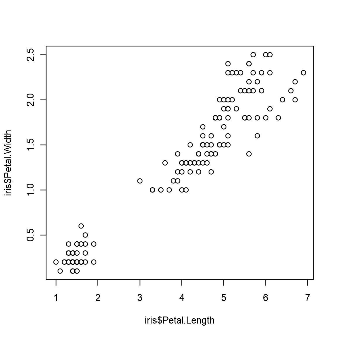
Below are some of chunk options relating to plots.
| Option | Default | Description |
|---|---|---|
| fig.height | 7 | Figure height in inches |
| fig.width | 7 | Figure width in inches |
| fig.cap | “” | Figure caption |
| fig.align | “center” | Figure alignment |
| dev | “png” | Change png,jpg,pdf etc |
2.6 Export
The R Markdown notebook can be exported into various format. The most common formats are HTML and PDF.
2.6.1 HTML
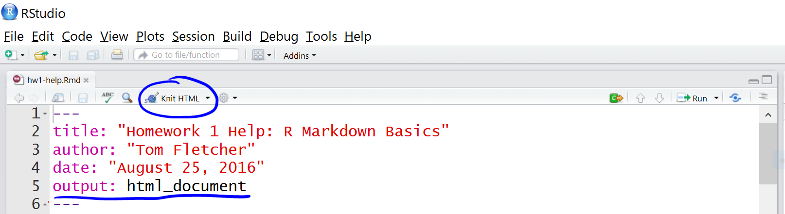
The R Markdown document can be previewed as an HTML inside RStudio by clicking the ‘Knit’ button.
The document can also be exported as an HTML file by running the code below:
rmarkdown::render("document.Rmd")HTML documents can be opened and viewed in any standard browser such as Chrome, Safari, Firefox etc.
2.6.2 PDF
An Rmd document can be converted to a PDF. Behind the scenes, the markdown is converted to TeX format. The conversion to PDF needs a tool that understands TeX format and converts to PDF. This can be softwares like ‘MacTeX’, ‘MikTeX’ etc. which needs to be installed on the system beforehand.
The output argument in the YAML matter must be changed to pdf_document, and the Rmd file can be converted as follows:
rmarkdown::render("document.Rmd")The PDF output can also be specified as such:
rmarkdown::render("document.Rmd",output_format=pdf_document())Sometimes TeX converters may need additional libraries which may need to be installed. And all features of HTML are not supported on TeX which may return errors.
See here for other export formats.
3 Challenges
3.1 Report
This is a do-it-yourself challenge to R Markdown Notebook/Report. Have a look at the HTML page below and try to recreate the page. Instructions and helpful tips are given below.
This is the challenge report to prepare.
- Create a new R Markdown document
- Set YAML matter
- Set title, subtitle, Author name.
- Set date to be automatically computed in this format “25/04/2018”. Refer to ‘YAML’ section above for how to do this. See here on how to format dates.
- Show a floating table of contents on the top left of the page. See here on how to do this.
- Set automatic numbering of sections.
- Set theme to ‘flatly’.
- Set code highlighting to ‘kate’.
- Notice the little buttons on the right to show/hide code. Show this button and set all code to hidden by default. See here on how to do this.
- Set the default data.frame printing option to pageable HTML table. See here.
- Add a Level 1 heading
- Add some text and a Level 2 heading
- Create an R chunk to display the structure of cars dataset. Display the code and the results. See here to read more about chunk options.
- Display the first six rows and all columns of the cars dataset as a table.
- Create a new sub-section and create a scatterplot with the two variables from cars dataset. Hide the code used and only show the plot. Create a square aspect ratio plot by setting equal figure height and width in the chunk options. Add a caption for the plot using chunk options.
- Create a new sub-section, download a random image and include it in the document.
- Render the document in RStudio by clicking on the ‘Knit’ button.
- Render the document to an HTML file using a console command.
- Render this document to a PDF. Change output type from
html_documenttopdf_documentand remove all arguments excepttoc: true. Try rendering using ‘Knit’.
3.2 Presentation | ioslides
This is a do-it-yourself challenge to ioslides Presentation using R Markdown. Have a look at the presentation below and try to recreate it. Instructions and helpful tips are given below.
This is the challenge ioslide presentation.
- Create a new R Markdown document.
- Set YAML matter output to
output: ioslides_presentation. See here for a guide to using ioslides presentation in R. - Set theme and highlight as needed.
- New slides are defined using
#with level 1 heading or----without a heading. Subtitle can be specified using a pipe symbol, like this# Title | Subtitle. Slides starting with#contains only the title and/or subtitle.##adds a standard content slide with a heading on the top. - Add a title slide
# Title Slide | Subtitle- Add a standard slide with a heading and a bulleted list. For example
## Level 2 Heading

- Point one
- Point two
The bullets can set to show incrementally on click:
## Level 2 Heading

> - Point one
> - Point two- Create a new slide and add some R chunk. For example:
```{r}
data(iris)
str(cars)
```- Create a new slide and display a table by executing an R chunk. For example:
```{r}
head(cars)
```- Create a new slide and display an R plot. For example:
```{r,fig.height=3,fig.width=5,fig.cap="This is a scatterplot."}
plot(cars$speed,cars$dist)
```- Add an image to a new slide. For example:
- When viewing the presentation, press
Oto see an overview of the slides.
3.3 Presentation | revealJS
This is a do-it-yourself challenge to RevealJS 2-D Presentation using R Markdown. Have a look at the presentation below and try to recreate it. Instructions and helpful tips are given below.
This is the challenge RevealJS presentation.
- Install R package
revealjsand load the library. - Create a new R Markdown document.
- Set YAML matter output to
output: revealjs::revealjs_presentation. See here for a guide to using RevealJS presentation in R. - Set theme and highlight as needed.
- New slides are defined using
#with level 1 heading,##with level 2 heading or----without a heading. The best feature of RevealJS is that slides are not restricted to horizontal (linear) flow. Slides can also flow vertical from any of the horizontal slides. A level 2 heading##signifies that the content under that flows vertically. - Add a level 1 heading and add some text content.
- Create a new slide vertically by adding a level 2 heading and add some R chunk. For example:
## Level 2 Heading

```{r}
data(iris)
str(cars)
```- Create a new slide vertically using level 2 heading and display a table by executing an R chunk. For example:
## Level 2 Heading

```{r}
head(cars)
```- Create a new slide vertically and display an R plot. For example:
## Level 2 Heading

```{r,fig.height=3,fig.width=5,fig.cap="This is a scatterplot."}
plot(cars$speed,cars$dist)
```- Create a new slide horizontally. Add an image to a new slide. For example:
- When viewing the presentation, press
Oto see an overview of the slides.
4 Session Info
- This document has been created in RStudio using R Markdown and related packages.
- For R Markdown, see http://rmarkdown.rstudio.com
- For details about the OS, packages and versions, see detailed information below:
sessionInfo()## R version 3.4.3 (2017-11-30)
## Platform: x86_64-w64-mingw32/x64 (64-bit)
## Running under: Windows >= 8 x64 (build 9200)
##
## Matrix products: default
##
## locale:
## [1] LC_COLLATE=English_United Kingdom.1252
## [2] LC_CTYPE=English_United Kingdom.1252
## [3] LC_MONETARY=English_United Kingdom.1252
## [4] LC_NUMERIC=C
## [5] LC_TIME=English_United Kingdom.1252
##
## attached base packages:
## [1] stats graphics grDevices utils datasets methods base
##
## other attached packages:
## [1] gdtools_0.1.7 bindrcpp_0.2 gridExtra_2.3 kableExtra_0.7.0
## [5] forcats_0.3.0 stringr_1.3.0 dplyr_0.7.4 purrr_0.2.4
## [9] readr_1.1.1 tidyr_0.8.1 tibble_1.4.2 ggplot2_2.2.1
## [13] tidyverse_1.2.1 captioner_2.2.3 bookdown_0.7 knitr_1.20
##
## loaded via a namespace (and not attached):
## [1] httr_1.3.1 jsonlite_1.5 viridisLite_0.3.0
## [4] R.utils_2.6.0 modelr_0.1.1 shiny_1.0.5
## [7] assertthat_0.2.0 highr_0.6 cellranger_1.1.0
## [10] yaml_2.1.19 pillar_1.2.2 backports_1.1.2
## [13] lattice_0.20-35 glue_1.2.0 uuid_0.1-2
## [16] digest_0.6.15 promises_1.0.1 rvest_0.3.2
## [19] colorspace_1.3-2 httpuv_1.4.1 cowplot_0.9.2
## [22] htmltools_0.3.6 R.oo_1.22.0 plyr_1.8.4
## [25] psych_1.8.3.3 xaringan_0.6 pkgconfig_2.0.1
## [28] broom_0.4.4 haven_1.1.1 xtable_1.8-2
## [31] scales_0.5.0.9000 later_0.7.2 officer_0.3.0
## [34] ggpubr_0.1.6 lazyeval_0.2.1 cli_1.0.0
## [37] mnormt_1.5-5 mime_0.5 magrittr_1.5
## [40] crayon_1.3.4 readxl_1.1.0 evaluate_0.10.1
## [43] R.methodsS3_1.7.1 nlme_3.1-137 xml2_1.2.0
## [46] foreign_0.8-70 Cairo_1.5-9 tools_3.4.3
## [49] data.table_1.11.0 hms_0.4.2 plotly_4.7.1
## [52] munsell_0.4.3 zip_1.0.0 compiler_3.4.3
## [55] rlang_0.2.0 grid_3.4.3 rstudioapi_0.7
## [58] htmlwidgets_1.2 crosstalk_1.0.0 base64enc_0.1-3
## [61] labeling_0.3 rmarkdown_1.9 gtable_0.2.0
## [64] reshape2_1.4.3 R6_2.2.2 rvg_0.1.8
## [67] lubridate_1.7.4 ggiraph_0.4.2 bindr_0.1.1
## [70] rprojroot_1.3-2 stringi_1.1.7 parallel_3.4.3
## [73] Rcpp_0.12.16 tidyselect_0.2.4 xfun_0.1Page built on: 28-May-2018 at 15:55:01.
2018 | SciLifeLab > NBIS > RaukR 
