3.1 Preparing the working environment

First, we need to prepare the working environment. To avoid typing long path names, we begin by setting our working directory using setwd() command. Next, we load GenABEL package using the library() command:

setwd("C:/Users/Nina/Documents/courses/R_summer_school/GWAStutorial/GWAS_Workshop/")
library(GenABEL)

3.2 Loading data

Now, we are ready to load genotyping data. These may come in a multitude of formats and GenABEL can read all common formats used in GWAS. To this end, GenABEL provides a number of conversion functions that translate data from a given file format to the internal GenABEL data structure. This internal data structure is optimized for access-time and memory usage and stores the data in a binary-compressed format. All the conversion functions are named in a uniform fashion starting with convert. For instance, convert.snp.ped() is a function that translates data from a common .ped format to GenABEL data structure. The genotyping data, once converted, is stored in a special file, typically with .raw extension. Phenotypes are stored in another file, in the form of a table. For details on both formats, type ?convert.snp.text() and ?load.gwaa.data(). Data is loaded using the load.gwaa.data() function which has some useful parameters. Two of these parameters are commonly used: makemap and sort. The first one is useful when the original genetic map is chromosome-specific, i.e., when marker coordinates are related to the beginning of chromosome. When set to makemap=TRUE, the coordinates will be translated to genome-wide map. The latter is helpful in the cases where markers are not sorted according to their order on chromosomes. Set sort=TRUE to sort markers according to their genomic coordinates. Having the parameters set, we can proceed and load the data:

# Load data
genodata <- load.gwaa.data(
            phenofile = "data/phenotype.dat", 
            genofile = "data/genotype.raw", 
            makemap = F, 
            sort = F)

3.3 Understanding the data structure

As mentioned in the previous subsection, GenABEL stores genetic data in a specific internal format gwaa.data. It is important to understand the structure of this format and how to access its parts. At its highest level, gwaa.data is a class consisting of two so-called slots: one slot for genotype data and one for phenotype data. These slots can be accessed by gtdata() (or @gtdata) and phdata() (or @phdata) selectors. Note that the selector(mydata) and mydata@selector are equivalent forms of notation and throughout this document, we will use them interchangeably to achieve as clear and compact notation as possible. Now, the genotype data is, in turn, of snp.data-class, which means you can access a list of chromosomes by writing mydata@gtdata@chromosome or chromosome(gtdata(mydata)) (or a combination of those two notations, e.g., chromosome(mydata@gtdata)). To learn about all the slots in the snp.data-class, simply type ?snp.data-class. The phenotype data is stored in the form of a data frame which is simply a table where each row corresponds to an individual and every column contains values of a trait or a variable, e.g. age at sampling. In order to see names of all the traits/variables you can issue the names(mydata@phdata) command.

Explore the above command and try them on the data, just be aware that especially the snp information is huge. Don’t hesitate to press the STOP button in the top-right corner of the terminal if the printed output gets too much.

3.4 Getting an overview of the data

Once the data are loaded, it is common the check some features of the dataset and learn more about variables. We begin by looking at the number of individuals and the number of markers in the data:

# Get information about number of individuals
nids(genodata)

## [1] 200

# Number of SNPs in the data
nsnps(genodata)

## [1] 729048

Get summary of the first 5 markers:

# Summary of the first 2 markers
summary(genodata@gtdata)[1:5, ]

Using the fact that column “Q.2” contains minor allele frequency (MAF) for each marker, we can easily plot MAF for, say, first 500 markers on chromosome 4.

chr4.idx <- which(genodata@gtdata@chromosome == 4)
maf <- summary(genodata@gtdata)[chr4.idx[1:500],"Q.2"]
plot(maf, type = 'l', main="MAF on chr 4", 
     xlab = "marker", ylab = "MAF", col = "slateblue")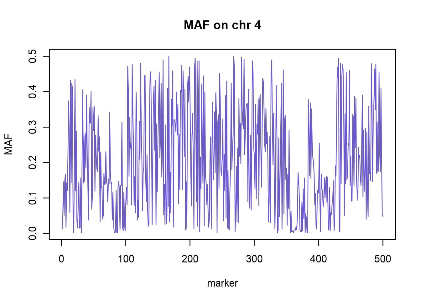

In a way similar to getting summary for genotype data, one can look at the phenotypes and other variables characterizing individuals. This is done as simply as issuing the summary command on the data frame containing phenotype information:

# Summary of phenotypes
summary(genodata@phdata)

##       id                 sex            pheno    
##  Length:200         Min.   :0.000   Min.   :0.0  
##  Class :character   1st Qu.:0.000   1st Qu.:0.0  
##  Mode  :character   Median :1.000   Median :0.5  
##                     Mean   :0.535   Mean   :0.5  
##                     3rd Qu.:1.000   3rd Qu.:1.0  
##                     Max.   :1.000   Max.   :1.0

As a result, R provides descriptive statistics per each trait. NOTE: Since R is assuming continuous nature of each variable, summary for binary traits like case/control or any variable taking discrete values is not helpful. However, if you want to view a table of your phenotypes, you can use the following, which will result in a searchable table:

# Make a table with all phenotypes per individual
library(DT)
datatable(genodata@phdata,options=list(pageLength=5))

3.5 Analyses of phenotypes

One of the first steps in the analyses is to identify potential dependencies between traits/variables as they should be taken into account when testing for accociations, e.g. males and females. To do this we use a Fisher’s exact test to test for association between sex and case control status.

TECHNICAL NOTE: We used attach(phdata(genodata)) to simplify notation. Now all the names within the genodata@phdata data frame can be referred just by their name, not by referring to the whole object, e.g., ab instead of genodata@phdata$ab. This is convenient, but in order to avoid confusion, remember to detach these names when you do not need them. We will do this later by writing detach(genodata@phdata).

attach(phdata(genodata))
#Binary trait analysis
tab <- table(pheno, sex)
rownames(tab) <- c("control","case")
colnames(tab) <- c("male","female")
tab

##          sex
## pheno     male female
##   control   43     57
##   case      50     50

fisher.test(tab)
detach(phdata(genodata))

## 
##  Fisher's Exact Test for Count Data
## 
## data:  tab
## p-value = 0.395
## alternative hypothesis: true odds ratio is not equal to 1
## 95 percent confidence interval:
##  0.4159816 1.3672058
## sample estimates:
## odds ratio 
##  0.7554638

Sex does not seem to be associated to case/control status. Now, we can continue with the quality control of the data.

3.6 Quality control

Quality control is one of the most crucial steps of the data analysis procedure. Be aware that any mistakes made at this step propagate and can seriously affect the results. Be careful! Quality control aims at removing poorly genotyped individuals and markers, markers that show large deviation from Hardy Weinberg equilibrium, markers with very low minor allele frequency and the individuals that are genetically too similar. In GenABEL, quality control is implemented in a convenient-to-use function check.marker(). The check.marker() function is implemented in an iterative manner: when, say, certain individuals are removed from the dataset due to low call rate, the size of the sample population changes and parameters like minor allele frequency have to be recalculated. The check.marker() function repeats data filtering until no further markers or individuals need to be removed. Typically, quality control takes two-three iterations of the check.marker() function. A typical call of check.marker() looks like this:

qc0 <- check.marker(genodata, call = 0.95, perid.call = 0.95, 
                    maf = 1e-08, p.lev = 1e-05, 
                    hweidsubset = genodata@phdata$pheno == 0)

## Excluding people/markers with extremely low call rate...
## 729048 markers and 200 people in total
## 0 people excluded because of call rate < 0.1 
## 0 markers excluded because of call rate < 0.1 
## Passed: 729048 markers and 200 people
## 
## RUN 1 
## 729048 markers and 200 people in total
## 0 (0%) markers excluded as having low (<1e-06%) minor allele frequency
## 934 (0.1281123%) markers excluded because of low (<95%) call rate
## 8 (0.001097321%) markers excluded because they are out of HWE (P <1e-05)
## 3 (1.5%) people excluded because of low (<95%) call rate
## Mean autosomal HET is 0.2990273 (s.e. 0.005555419)
## 0 people excluded because too high autosomal heterozygosity (FDR <1%)
## Mean IBS is 0.7463368 (s.e. 0.007302501), as based on 2000 autosomal markers
## 0 (0%) people excluded because of too high IBS (>=0.95)
## In total, 728106 (99.87079%) markers passed all criteria
## In total, 197 (98.5%) people passed all criteria
## 
## RUN 2 
## 728106 markers and 197 people in total
## 223 (0.03062741%) markers excluded as having low (<1e-06%) minor allele frequency
## 105 (0.01442098%) markers excluded because of low (<95%) call rate
## 1 (0.0001373426%) markers excluded because they are out of HWE (P <1e-05)
## 0 (0%) people excluded because of low (<95%) call rate
## Mean autosomal HET is 0.2990772 (s.e. 0.005581424)
## 0 people excluded because too high autosomal heterozygosity (FDR <1%)
## Mean IBS is 0.7516317 (s.e. 0.006968945), as based on 2000 autosomal markers
## 0 (0%) people excluded because of too high IBS (>=0.95)
## In total, 727777 (99.95481%) markers passed all criteria
## In total, 197 (100%) people passed all criteria
## 
## RUN 3 
## 727777 markers and 197 people in total
## 0 (0%) markers excluded as having low (<1e-06%) minor allele frequency
## 0 (0%) markers excluded because of low (<95%) call rate
## 0 (0%) markers excluded because they are out of HWE (P <1e-05)
## 0 (0%) people excluded because of low (<95%) call rate
## Mean autosomal HET is 0.2990772 (s.e. 0.005581424)
## 0 people excluded because too high autosomal heterozygosity (FDR <1%)
## Mean IBS is 0.7512698 (s.e. 0.007531951), as based on 2000 autosomal markers
## 0 (0%) people excluded because of too high IBS (>=0.95)
## In total, 727777 (100%) markers passed all criteria
## In total, 197 (100%) people passed all criteria

It is important to fully understand all the parameters of the function and to adjust them according to the type of analyzed data, studied organism, purpose of the study etc. Below we provide a brief discussion of the most relevant parameters, for further information, refer to the function manual by typing ?check.marker():

• Poorly genotyped markers are defined in terms of call rate. Setting threshold callrate = 0.95, results in filtering out the markers that have missing genotype in 5% or more individuals. The 0.95 threshold is a reasonable value in most cases, but it is important to remember that it is specific to genotyping technology, version of array etc. Therefore always refer to manufacturer’s guidelines when in doubt.

• Similarly to poorly genotyped markers, also the poorly genotyped individuals can be filtered out. Setting perid.call=0.95 will result in filtering out the individuals with 5% or more missing genotypes. Likewise in the previous point, values of 0.95 or even 0.98 are usually appropriate but when in doubt, consult appropriate manuals and guidelines of the genotyping array manufacturer.

• By default, markers and individuals with extremely low call rate (10%) are dropped prior to the iterative quality control. These thresholds are set by extra.call and extra.perid.call parameters but in the vast majority of analyses they should be left at their default levels.

• Individuals showing abnormally high level of heterozygosity are filtered out using the het.fdr threshold. Departure from expected heterozygosity is measured and the threshold is defined in terms of false discovery rate (FDR). At the default level het.fdr = 0.01, one accepts that 1% of the individuals filtered out due to unacceptably high heterozygosity may not in fact be true outliers.

• In many data analysis scenarios, removal of genetically identical or too similar individuals is an important part of the quality control procedure. Redundancy and high correlation in the data can result in an overly inflation of the results. Therefore, too similar individuals should be identified and either removed or treated with care. Roughly, the genetic similarity between a pair of individuals is measured by the number of loci at which these individuals differ. The degree of similarity is expressed in terms of average identity-by-state (IBS). ibs.threshold parameter sets a cut-off value for the degree of similarity between any pair of individuals. Unless using experimental design with very related individuals, the default value of ibs.threshold = 0.95 should be used which assures that individuals with genomic similarity of 95% or more will be treated as too related. This would assure that all potential duplicates are removed, as well as any potential monozygotic twins. Later on we will also remove first and second degree relatives. Computing IBS on the basis of all available markers would be computationally very demanding, therefore the actual IBS computations are based on a randomly selected subset of all markers. Typically the default 2000 markers should be more than enough, but if required, this value can be changed by setting ibs.mrk parameter. To turn off IBS checks set ibs.mrk = -1 and to use all markers set ibs.mrk = “all”. When IBS exceeds the ibs.threshold, either both individuals ibs.exclude = “both” can be removed from the dataset or only the one with lower call rate ibs.exclude = “lower”. One can also decide to keep both ibs.exclude = “none”. It is recommended to use none of the first two options.

• The maf parameter is controlling cut-off value for removing markers with low minor allele frequency (MAF). In a typical GWAS study, it is customary to set MAF threshold to 5% or even 1% (maf = .05 or maf = 0.01 respectively). At the preliminary quality control step one may be willing to remove the non-informative (monomorphic) markers only which can be accomplished by setting maf = 1e-06.

• Markers can be filtered out based on the degree of departure from HardyWeinberg equilibrium (HWE). Departure from HWE is tested using goodness-of-fit \(\chi^2\) test. By default, parameter p.level sets the cut-off value in terms of p-value; when is set to a negative value, e.g. p.value = -1, FDR-based cut-off specified by the fdrate parameter is used. While strong departures from HWE may be due to a systematic genotyping error, in certain scenarios it is important to allow for higher departures from HWE in a subset of individuals. Case-control is a good example of such set-up - a departure from HWE at a disease locus may, under certain conditions be expected in cases. Due to this it is most common to only use controls when testing for deviation from HWE. It is possible to specify the subset of individuals to be tested for departures from HWE using the hweidsubset parameter (specify individuals by either their names, indices or using a logical vector). The most commonly used threshold for HWE are p < 1e-6 or p < 1e-8.

• There is more parameters of the check.marker() function that allow for precise control of the quality control process, in particular for sexchromosome checks, redundancy-checks and heterozygosity-checks. As these parameters do not have to be set in a typical analysis, we skip the detailed discussion and send the reader to the GenABEL documentation.

3.7 On interpreting the quality control results

Now the preliminary quality control is completed. Please observe that at each round of the iterative process, some markers and individuals were excluded based on the criteria we set. A comprehensive overview of the outcome can be easily produced:

summary(qc0)

## $`Per-SNP fails statistics`
##           NoCall NoMAF NoHWE Redundant Xsnpfail
## NoCall      1039     0     0         0        0
## NoMAF         NA   223     0         0        0
## NoHWE         NA    NA     9         0        0
## Redundant     NA    NA    NA         0        0
## Xsnpfail      NA    NA    NA        NA        0
## 
## $`Per-person fails statistics`
##             IDnoCall HetFail IBSFail isfemale ismale isXXY otherSexErr
## IDnoCall           3       0       0        0      0     0           0
## HetFail           NA       0       0        0      0     0           0
## IBSFail           NA      NA       0        0      0     0           0
## isfemale          NA      NA      NA        0      0     0           0
## ismale            NA      NA      NA       NA      0     0           0
## isXXY             NA      NA      NA       NA     NA     0           0
## otherSexErr       NA      NA      NA       NA     NA    NA           0

We can see that, for instance, 223 markers were excluded due to being monomorphic in our data, and 1039 markers were excluded due to too low call rate. There is no rule of thumb as to how many markers and individuals should pass quality control, it depends on species, genotyping technology used, and experimental design. It is up to the researcher to decide whether the observed data quality is satisfactory to carry on further analyses. In our analysis we can also see that 3 individuals were excluded due to too many missing calls. The reasons why this happens could be many; DNA quality migth not be good enough, they might come from genotyping chips that were suboptimal, reagents were old, or there may be a batch effect caused by something in the genotyping process. Always try to investigate why the samples failed before removing them.

Once the quality control is completed, the results are stored in a special object of check.marker-class class. If you need to know which particular markers of individuals were excluded due to a given reason, you can get this information by accessing appropriate slots of the object stored in the qc0 variable. More information on the structure of the object can be obtained by typing ?check.marker-class. Running the check.marker only points out the problems but does not alter the actual data. Once the problematic markers and individuals are identified, they can be removed from the dataset:

genodata.qc0 <- genodata[qc0$idok, qc0$snpok]

3.8 Detection and analyses of population stratification

After preliminary quality control, it is time to examine structure of the analysed population, detect potential genetic outliers and look at the degree of relatedness between individuals. The first step is to create a genomic kinship matrix - a \(\sf{N_{i}nd x N{i}_ind}\) matrix which reflects the degree of genetic similiarity between an pair from \(\sf{N_{i}nd}\) individuals.

NOTE: To avoid unwanted bias, computation of the genomics kinship matrix should be based on the autosomal markers only. When working with human data, the autosomal(genodata.qc0) function can be used to retrieve the names of all autosomal markers. When working with other species, it is the user who has to define the subset of autosomal markers based on chromosome number. As our dataset is simulated using the 1000G data, we don’t have any sex chromosomes present in the data, but for future reference we will still perform the selection of autosomal markers first:

autosomalMarkerNames <- autosomal(genodata.qc0)
# Compute genomic kinship matrix
genodata.qc0.gkin <- ibs(genodata.qc0[, autosomalMarkerNames], weight = "freq")
# Transform it to a distance matrix
genodata.qc0.dist <- as.dist(0.5 - genodata.qc0.gkin)
# Perform multidimensional scaling to display individuals on a 2D
genodata.qc0.pcs  <- cmdscale(genodata.qc0.dist, k=10)
# Label the samples according to case control status
genodata.qc0.pcs <- cbind(genodata.qc0.pcs, genodata.qc0@phdata$pheno)
# Plot the result
{plot(x=genodata.qc0.pcs[, 1], y=genodata.qc0.pcs[, 2], xlab = "PC 1", ylab = "PC 2",
      col=c("grey","slateblue")[as.factor(genodata.qc0.pcs[, 11])], main = "Genomic kinship")
legend(x=0.06,y=0.09,legend=c("control","case"),
       col=c("grey","slateblue"),pch=19)}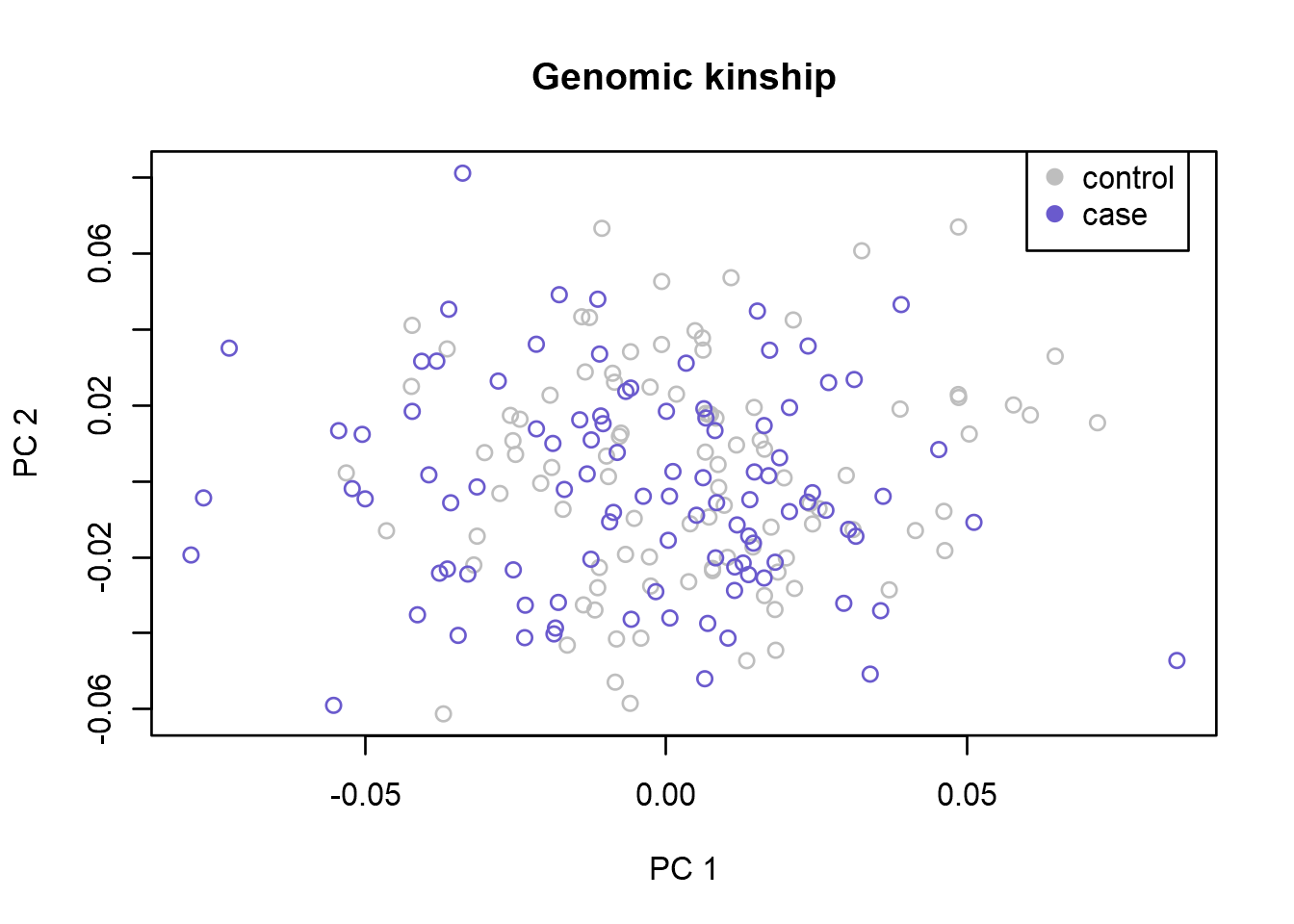

The plot shows a two-dimensional visualization of the computed genomic-kinship matrix where every individual is represented as a point. Here we can see Principal Components (PCs) 1 versus 2, but make sure to also study other PCs for outliers. When studying the plots, look for any samples that does not cluster with the others, and study how well cases and controls overlap. Having outliers in your data, and an unbalanced case control population will cause stratification issues in your analysis. This might lead to inflation and possible false positive results. That is why it is important to identify and remove outliers, and correct for stratification issues. Once you have identified outliers, remove them using the identify function. Use ?identify to read more about how it works. In this data we don’t have any obvious outliers, so we will not remove any samples.

In our initial QC we computed IBS and removed any duplicate samples. However, to avoid inflation in our results, in most association studies it is important to remove samples that are too closely related. The most common approach is to remove one sample in a pair that is more closely related then second degree relatives. To test for relatedness we will use the findRelatives function, and specify it to look for any relations up to 4 meosis apart (3 meosis apart corresponds to second degree relatives). Before doing this, we will randomly select 5,000 markers to run the test on, as we don’t want too many markers that are in linkage disequillibrium (LD):

# Subsample 5,000 SNPs that will be used for analysis
genodata.qc0.sub <- genodata.qc0[,sort(sample(1:nsnps(genodata.qc0),5000))]
# Extract allele frequencies
eaf <- summary(gtdata(genodata.qc0.sub))$"Q.2"
# Find relatives
relInfo <- findRelatives(genodata.qc0.sub,q=eaf,gkinCutOff=-1,nmeivec=c(1,2,3,4))

# Summarize the guesses made by the function
summary(relInfo$compressedGuess)

## < table of extent 0 x 0 >

These results displaying an empty table indicates that we have no pairs of samples that are closer than 4 meiosis apart. As we had no obvious outliers from the PCA analysis in the previous step either, we can proceed with our data as it is.

3.9 Testing for associations

Once we know our data is of good quality, it is time to perform the genome-wide association study (GWAS). In our setup we will analyze a binary trait and find markers associated with our imaginary Disease X. To accomplish this, we will test marker by marker using a statistical test (Cochran-Armitage trend test). This is implemented in GenABEL as qtscore() function.

# Build the model and test for association
an <- qtscore(pheno, genodata.qc0, trait="binomial")

Now the results of all the tests are stored in the “an” object. We can plot per-marker p-values using a Manhattan plot:

# Plot results
plot(an, col=c("olivedrab","slateblue"), cex=.5, main="Manhattan plot")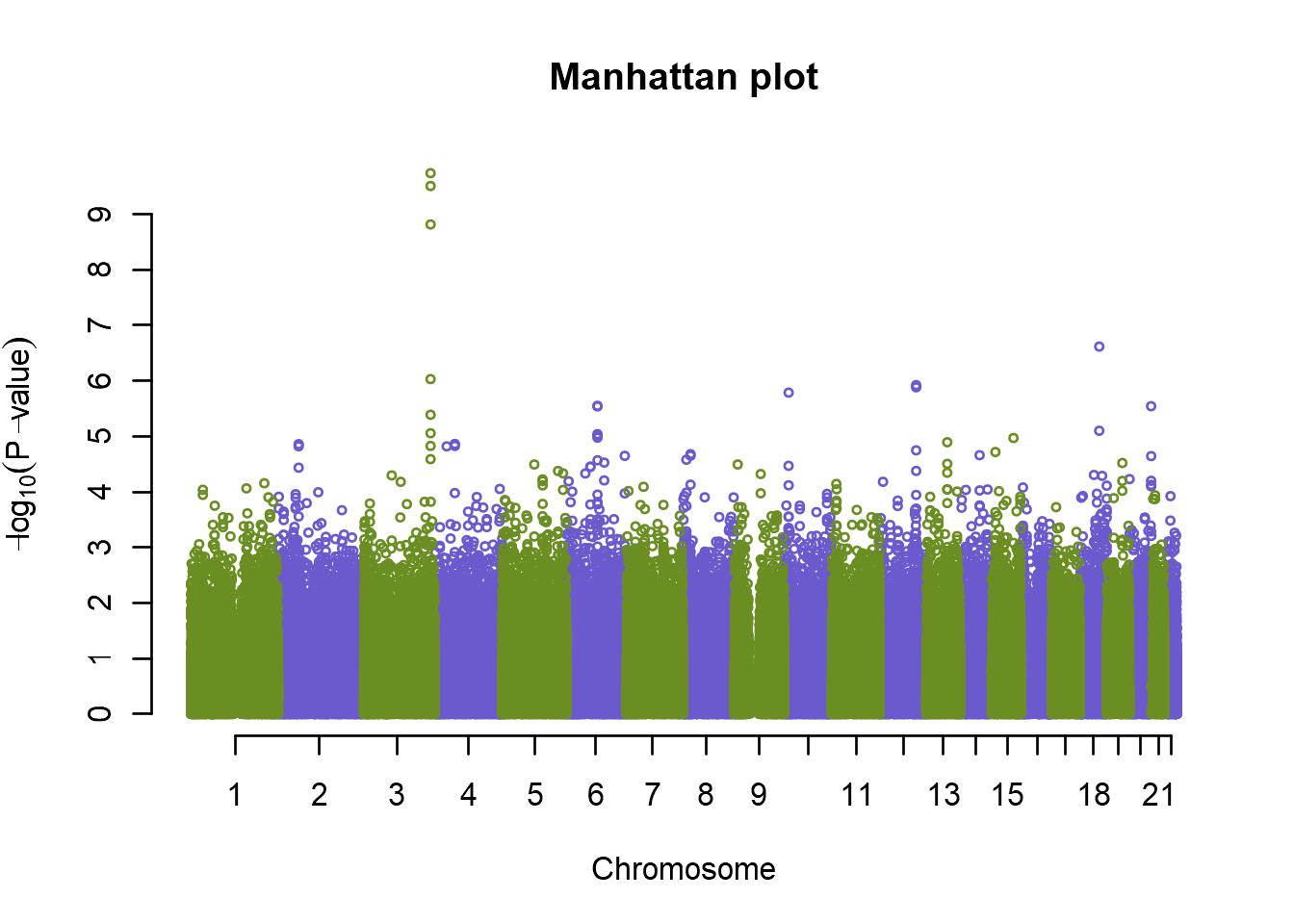

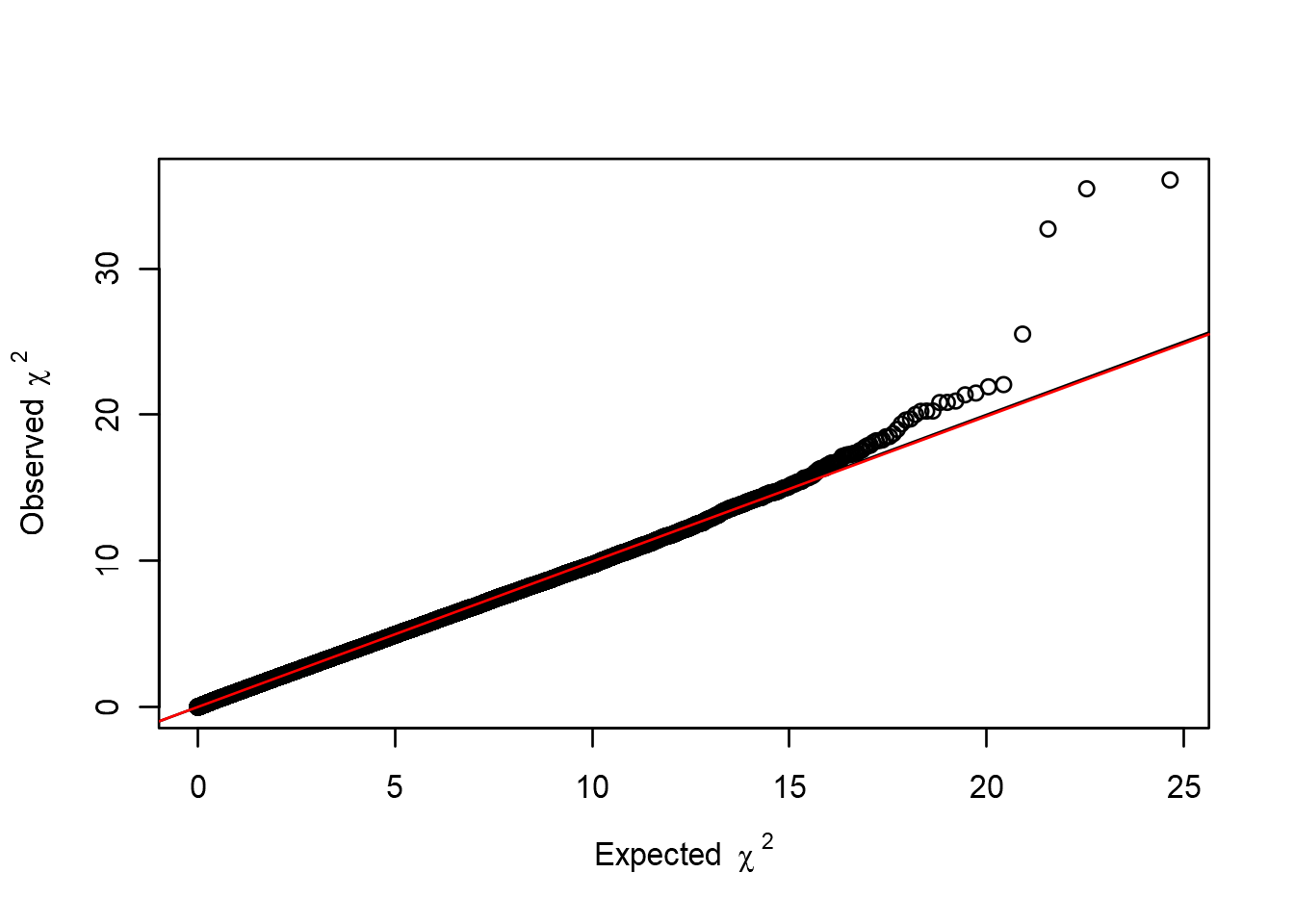
So it appears we have an association on chromosome 3, but before we start to celebrate let’s look at bit closer at the genomic inflation factor, \(\lambda\), first. If we have a lot of cryptic relatedness, or population stratification issues in our data, as investigated in our QC, the genomic inflation factor will be affected. If \(\lambda\) is greater than 1, it means we have more low p-values than expected. Let’s examine \(\lambda\) and see how our p-values are distributed compared to the theoretical distribution. We can use a Q-Q plot to accomplish this:

# Calculate lambda for results
estlambda(an[, "P1df"], plot=TRUE)

## $estimate
## [1] 1.004447
## 
## $se
## [1] 3.747573e-05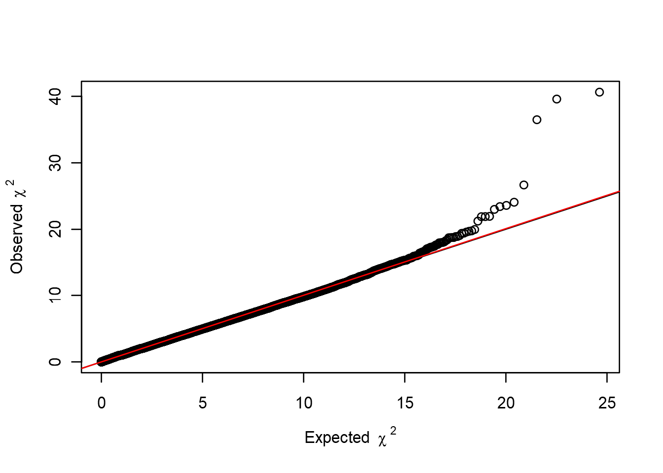

So in our example \(\lambda\) is quite close to 1, and we wouldn’t expect any major impact on our association results. But in cases where \(\lambda\) is higher than 1, we have to correct our association analysis for this. What value of \(\lambda\) is considered too high then? There is no consensus, but if the \(\lambda\) values start to be higher than 1.04-1.05 you should probably correct for stratification. There are a few ways of doing this correction. The most common approach in human genetics is to include the first 10 principal components as covariates.

an.pca <- qtscore(pheno~genodata.qc0.pcs[, 1:10], genodata.qc0, trait="binomial")
plot(an.pca, col=c("olivedrab","slateblue"), cex=.5, main="Manhattan plot")
estlambda(an.pca[, "P1df"], plot=TRUE)

## $estimate
## [1] 0.9949179
## 
## $se
## [1] 2.571614e-05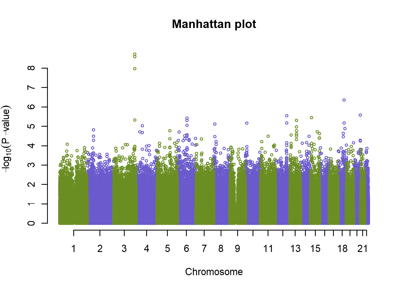

Looking at our Manhattan plot we see that the p-values have now been adjusted for population stratification, and \(\lambda\) has dropped to just below 1.

So now we have one peak at chromosome 8 that looks significant, and some other peaks that might also be of interest, but are they really statistically significant? In human genetics studies, the genome wide association p-value limit is usually agreed upon to be \(\sf{5e^{-8}}\). So let’s first summarize our top SNPs, and also add a significance line to our plot:

plot(an.pca, col=c("olivedrab","slateblue"), cex=.5, main="Manhattan plot")
abline(h = -log10(5e-8), col = "red")
summary(an.pca)

## Summary for top 10 results, sorted by P1df

Congratulations! You just discovered a new loci associated with Disease X. Your next step would now be to look into any potential genes in this region, and use annotations to search for candidate markers that could be causal. Remember that just because on of the markers came out more significant than the others, it doesn’t mean that that is the causal marker. LD in the region means that the causal marker might just be in LD with the top hit. After this you would optimally set up a validation study to try to replicate the results, and possibly do functional studies.

A NOTE ON CORRECTION FOR MULTIPLE TESTING:

Although in human genetics studies the significance level has been agreed upon, that is not the case in many other non-human studies. A simple approach to account for multiple testing would be to use Bonferroni correction, simple dividing the significant p-value with the number of markers tested. In our data set that would be:

# Calculate the Bonferroni threshold
bonferroni <- -log10(0.05/nsnps(genodata.qc0))
# Add the line to our plot
plot(an.pca, col=c("olivedrab","slateblue"), cex=.5, main="Manhattan plot")
abline(h = bonferroni, col = "red")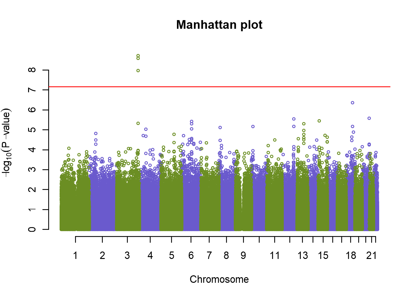

Here we can see that the singificance line does not change that much. However, if you have imputed data with 5 million plus markers, the Bonferroni correction would be much too conservative. The best option would then be to run permutation tests, to get the right estimate of the true significance level. Permutation test is a test where we randomly shuffle phenotypic values and perform the same assocation test as for the original data. We do this several (typicalle several thousand) times and record the “best”, i.e. the lowest p-value from each run. The position of our original best p-value on the distribution of the best p-values obtained with permuation test allows us to assess the true chance of committin type-I errors. Permutation test is very easy to perform in GenABEL, but can take significant amount of time. Therefore we just show how to call it:

# Perform 10,000 permutation tests
an.pca.per <- qtscore(pheno~genodata.qc0.pcs[, 1:10], genodata.qc0, trait="binomial", times = 10000)

THANK YOU AND GOOD LUCK WITH YOUR FUTURE GWAS STUDIES