ggmap
Plotting with maps
Sebastian DiLorenzo
11-Jun-2018
![]()
This exercise will show you how to use ggmap to produce maps and combine them with data and the ggplot2 skills you have learned for geospatial visualisation.
1 Installing requirements
Lets start by installing and loading the required packages. Note that we are using the github version of ggmap. If you have already installed some of the packages you can skip those.
2 Maps | get_map() and ggmap()
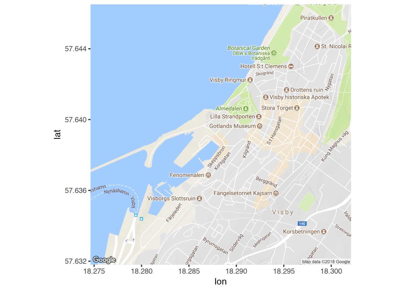
As the name suggests, the get_map function from ggmap is used to get maps. The maps are of the class ggmap and you can get many different maptypes.
- Use
ggmap(), the function, to plot a ggmap object created byget_mapand try out a few maptypes.
Note: Unless you have adjusted
ggmapsettings with a google API key theget_mapseems to be a bit unreliable during testing. If the command fails, try again a few times. Save it to a variable so you don’t have to keep querying the map servers.
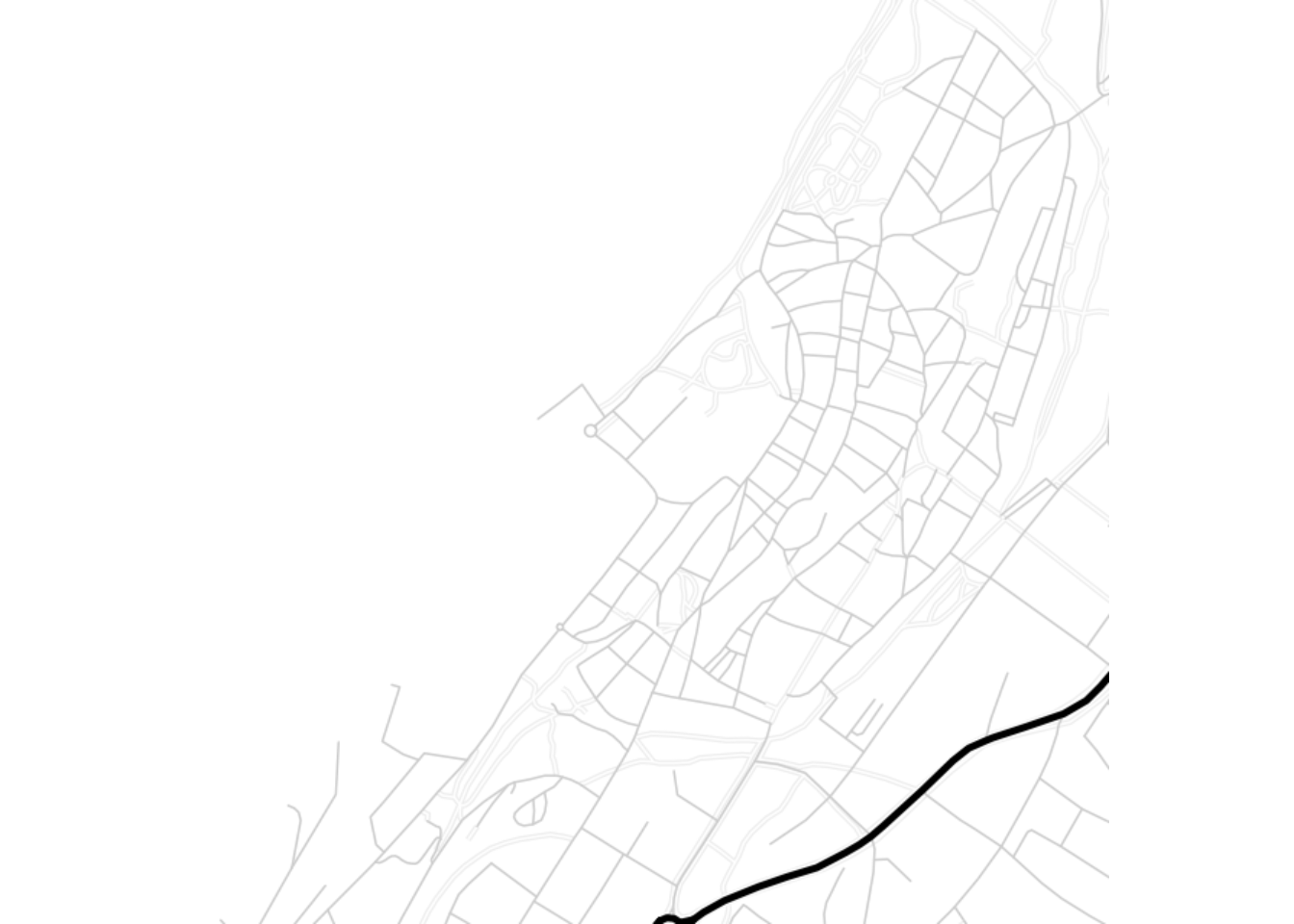
Trying out some other maptypes:
visby.watercolor.map <- get_map("Campus Gotland, Visby", zoom = 15, maptype = "watercolor")
visby.tonerlines.map <- get_map("Campus Gotland, Visby", zoom = 15, maptype = "toner-lines")

#extent="device" : removes long/lat axes
ggmap(visby.watercolor.map, extent="device")
ggmap(visby.tonerlines.map, extent="device")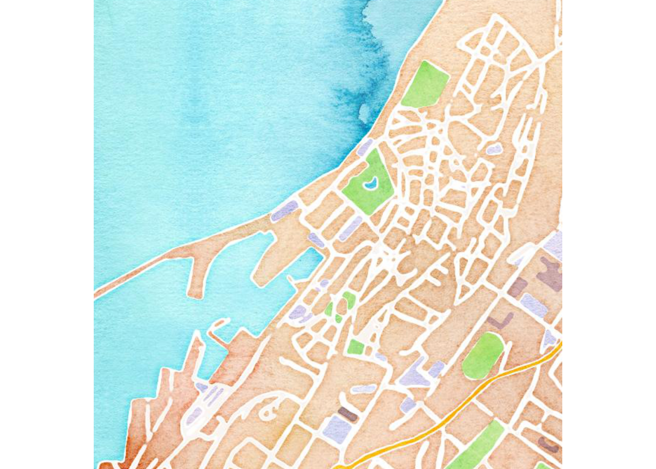
3 Add data to the map
Being able to output maps is great but, as with everything in life, it becomes more interesting when you can overlay it with data.
3.1 Points | geocode() and geom_point()
ggmap::geocode() is a nifty function that returns the latitude and longitude of a location. Use this to get the geocode of a place within the map that you created earlier in the exercise. Your favourite gym or restaurant for example?
In my example code, I show how to use tibble to get geocodes for several locations and bind them together to a data.frame.
#Create a tibble of Visby's most important locations
visby.locations <- tibble(location = c("Mullbärsgården, Visby",
  "Visby Hostel, Visby",
  "Glassmagasinet, Visby"))

#Get the geocode, the latitude and longitude, of the locations
visby.geo <- geocode(visby.locations$location)

#Create a data.frame of the data for easier plotting
visby.places <- cbind(visby.locations,visby.geo)
When you have your locations dataset ready, use geom_point to add markers to your map for your locations. Feel free to use geom_text to also add labels for your locations. Notice that you can treat the ggmap function like ggplot.
ggmap(visby.watercolor.map, extent="device") +
  geom_point(data = visby.places, aes(x = lon, y = lat), color = 'red', size = 3) +
  geom_text(data = visby.places, aes(label = location), hjust=0, vjust=-1)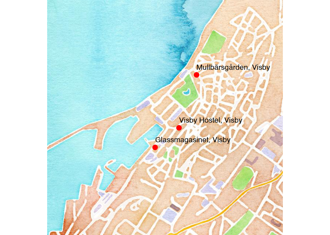
3.2 Routes | trek() and geom_path()
trek is a function from ggmap that takes a start location and a stop location and gives a list of latitude and longitude coordinates connecting the two. You can give several different modes of transit, but why anyone would choose anything other than bicycling is beyond me.
Combining trek and ggplot2 geom_path we can plot a route between two places, as long as one exists. Regrettably it doesn’t seem like airplane transits are included yet. Read the help page for trek and try it out.
Note: Make sure your background map covers both start and stop position!
#Create a map that is zoomed out enough to show start and stop of route
visby.zoomedout.map <- get_map("Visby", zoom = 7)

#Create the route with trek()
sthlm_vby <- trek("Stockholm, Sweden", "Visby, Sweden",
  structure = "route", mode = "bicycling")

#Plot the route to map
ggmap(visby.zoomedout.map, extent="device") +
  geom_path( aes(x = lon, y = lat),  colour = "blue",
    size = 1.5, alpha = .5,
    data = sthlm_vby, lineend = "round")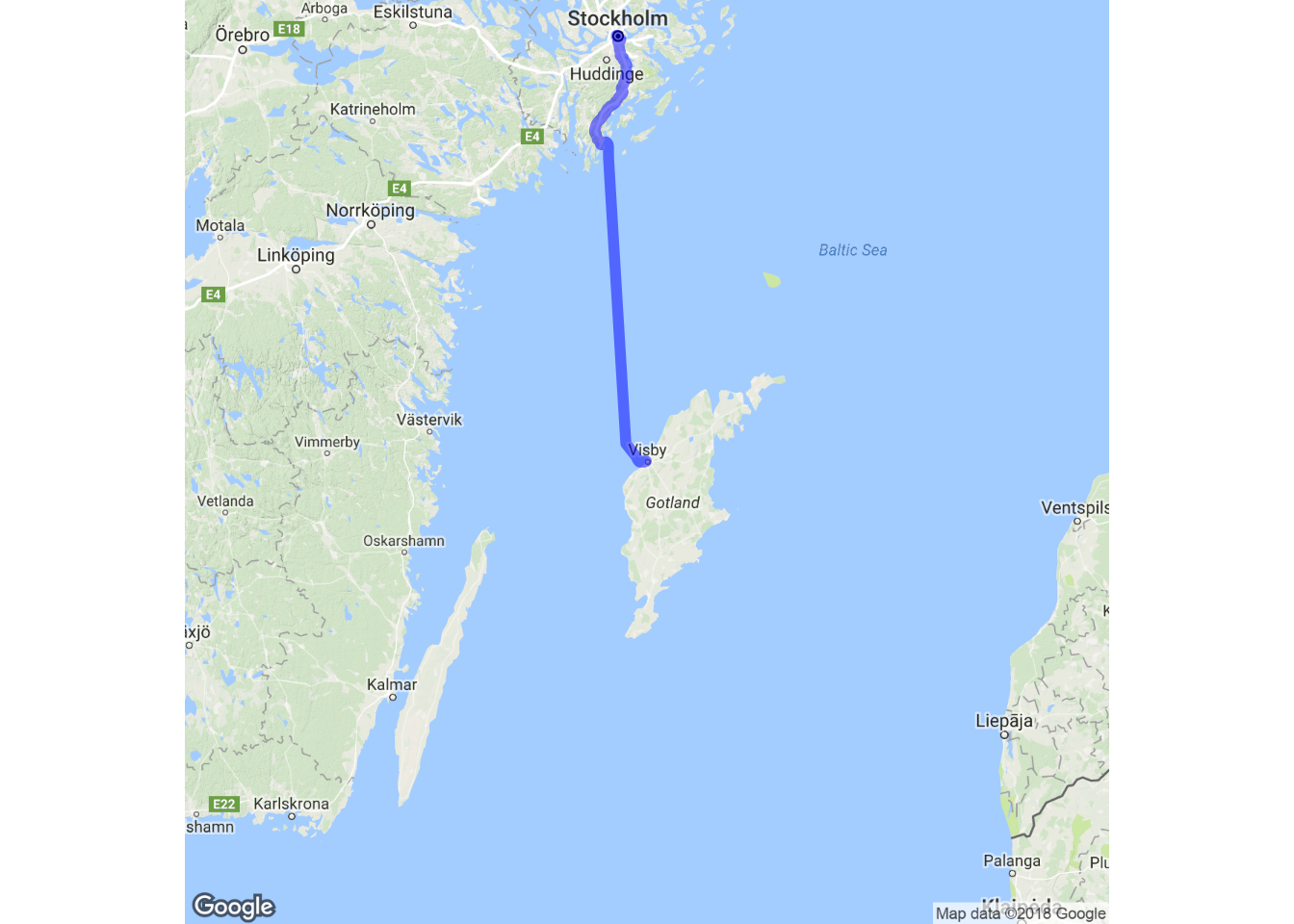
3.3 Pubs
What do they mean by pubs? Do they mean publications? Nope! We are going to plot actual pubs, bars, inns in the UK using a public dataset from https://www.getthedata.com/open-pubs.
Download the dataset pubs.rda from course materials.
Note: I have processed this data slightly, to see how unhide the following code box.
#Read the dataset
pubs <- read.csv("open_pubs.csv", stringsAsFactors = F)

#Set column names
colnames(pubs) <- c("fsa_id","name","address","postcode","easting","northing",
  "latitude","longitude","city")

#Convert long/lat to numeric
pubs$latitude <- as.numeric(pubs$latitude)
pubs$longitude <- as.numeric(pubs$longitude)

#Remove any rows with NA values
pubs <- pubs[complete.cases(pubs),]
Use what you have learned so far to complete as many tasks as you have time for. There is some help code and example plots of the town “Oldham” below, but really try to do it yourself before you unhide it.
- Load
pubs.rdainto R. - Subset the dataset to a city.
- Get a map of the city with
ggmap. - Plot the position of the pubs onto the map using
geom_point. - Create another plot where you plot the density lines of pubs using
geom_density2d.
- Optional: Feel free to select an appropriate maptype that isn’t so busy with text, I suggest the darker toner ones.
- Fill the density lines by overlaying with
stat_density_2das well. Use parametergeom = "polygon".
- Tip: You can use
scale_fill_gradient2andscale_alphato adjust colors and alpha.
Example code: Don’t unhide unless you’ve tried!
Task 4:
ggmap(oldham.map, extent="device") +
  geom_point(data = oldham.pubs, aes(x = longitude, y = latitude),
    color = 'red', size = 2)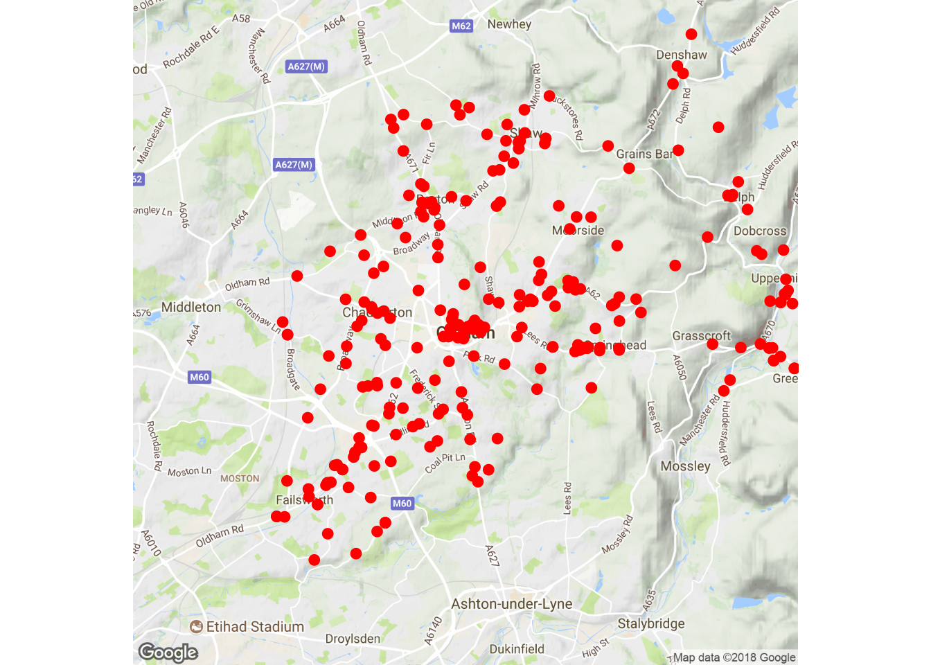
Task 5:
ggmap(oldham.toner.map, extent="device", darken = .7, legend = "bottomright") +
  geom_density2d(data = oldham.pubs, aes(x = longitude, y = latitude))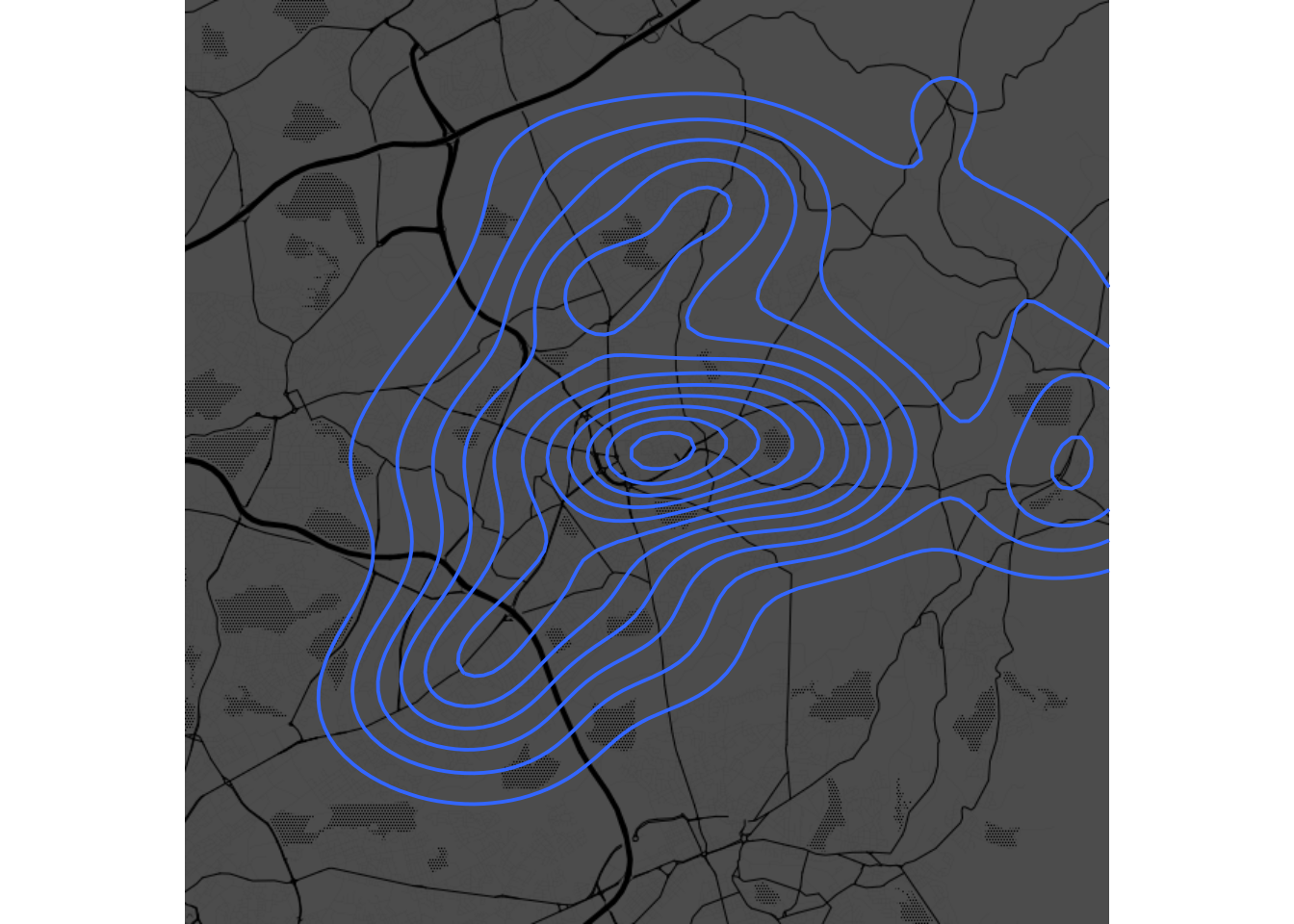
Task 6:
ggmap(oldham.toner.map, extent="device", darken = .7, legend = "bottomright") +
  geom_density2d(data = oldham.pubs, aes(x = longitude, y = latitude)) +
  stat_density_2d(data = oldham.pubs, aes(x = longitude, y = latitude,
    fill = ..level..,alpha = ..level..), geom = "polygon", color = NA)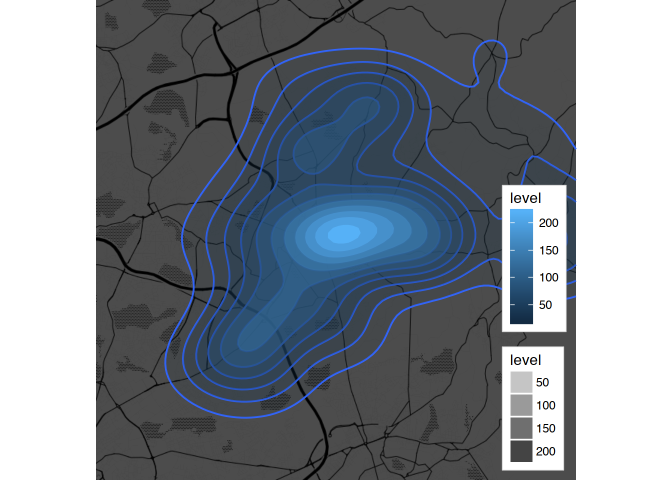
Task 6, tweaked:
ggmap(oldham.toner.map, extent="device", darken = .7, legend = "bottomright") +
  # Commenting geom_density2d, it is prettier without the lines =)
  #geom_density2d(data = oldham.pubs, aes(x = longitude, y = latitude)) +
  stat_density_2d(data = oldham.pubs, aes(x = longitude, y = latitude,
    fill = ..level..,alpha = ..level..), geom = "polygon", color = NA) +
  scale_fill_gradient2("Pubs", low = "white", mid = "yellow",
    high = "red", midpoint = 125) +
  scale_alpha(range = c(0.05, 0.30), guide = FALSE)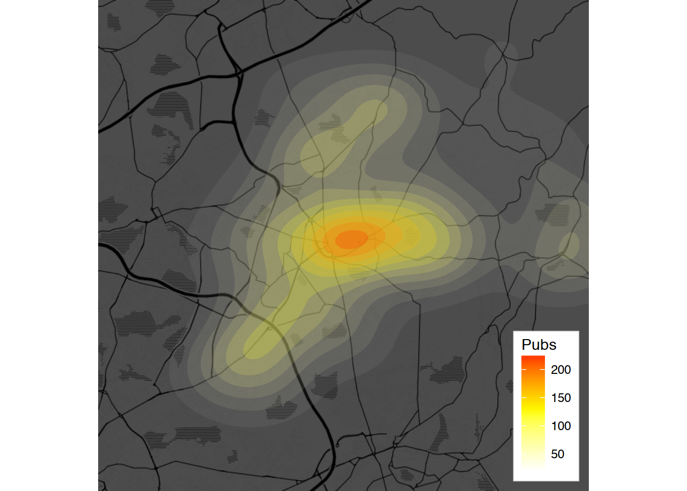
4 Session Info
- This document has been created in RStudio using R Markdown and related packages.
- For R Markdown, see http://rmarkdown.rstudio.com
- For details about the OS, packages and versions, see detailed information below:
## R version 3.5.0 (2018-04-23)
## Platform: x86_64-apple-darwin16.7.0 (64-bit)
## Running under: macOS High Sierra 10.13.4
##
## Matrix products: default
## BLAS: /System/Library/Frameworks/Accelerate.framework/Versions/A/Frameworks/vecLib.framework/Versions/A/libBLAS.dylib
## LAPACK: /System/Library/Frameworks/Accelerate.framework/Versions/A/Frameworks/vecLib.framework/Versions/A/libLAPACK.dylib
##
## locale:
## [1] en_US.UTF-8
##
## attached base packages:
## [1] stats     graphics  grDevices utils     datasets  methods   base
##
## other attached packages:
##  [1] bindrcpp_0.2.2  ggmap_2.7.900   forcats_0.3.0   stringr_1.3.1
##  [5] dplyr_0.7.5     purrr_0.2.5     readr_1.1.1     tidyr_0.8.1
##  [9] tibble_1.4.2    ggplot2_2.2.1   tidyverse_1.2.1 captioner_2.2.3
## [13] bookdown_0.7    knitr_1.20
##
## loaded via a namespace (and not attached):
##  [1] tidyselect_0.2.4  xfun_0.1          reshape2_1.4.3
##  [4] haven_1.1.1       lattice_0.20-35   colorspace_1.3-2
##  [7] htmltools_0.3.6   yaml_2.1.19       rlang_0.2.1
## [10] pillar_1.2.3      foreign_0.8-70    glue_1.2.0
## [13] modelr_0.1.2      readxl_1.1.0      jpeg_0.1-8
## [16] bindr_0.1.1       plyr_1.8.4        munsell_0.4.3
## [19] gtable_0.2.0      cellranger_1.1.0  rvest_0.3.2
## [22] RgoogleMaps_1.4.2 psych_1.8.4       evaluate_0.10.1
## [25] labeling_0.3      Cairo_1.5-9       parallel_3.5.0
## [28] broom_0.4.4       Rcpp_0.12.17      backports_1.1.2
## [31] scales_0.5.0      jsonlite_1.5      mnormt_1.5-5
## [34] rjson_0.2.19      png_0.1-7         hms_0.4.2
## [37] digest_0.6.15     stringi_1.2.2     grid_3.5.0
## [40] rprojroot_1.3-2   bitops_1.0-6      cli_1.0.0
## [43] tools_3.5.0       magrittr_1.5      lazyeval_0.2.1
## [46] crayon_1.3.4      pkgconfig_2.0.1   MASS_7.3-49
## [49] xml2_1.2.0        lubridate_1.7.4   rstudioapi_0.7
## [52] assertthat_0.2.0  rmarkdown_1.9     httr_1.3.1
## [55] R6_2.2.2          nlme_3.1-137      compiler_3.5.0
Page built on: 11-Jun-2018 at 14:23:21.
2018 | SciLifeLab > NBIS > RaukR

