Machine Learning in R

class: center, middle, inverse, title-slide

# Machine Learning in R
## Advanced R for Bioinformatics. Visby, 2018.
### Nikolay Oskolkov
### 18 juni, 2018

---

class: spaced

## Data Science and Artificial Intelligence

* The world’s most valuable resource is no longer oil, but Data
* Big Data is arriving, Bioinformatics learns from Data Science
* Data Science speaks predominantly Python, Scala and R
* Apache Spark, Probabilistic Programming and AI become common

![Oil vs. Data](Oil_vs_Data.jpg)

---
name: Data Science and Artificial Intelligence

## What is Machine Learning?

* Machine Learning maps input X to output Y as
`$$Y = f ( X )$$`
without necessarily knowing the functional form of f

* Machine Learning provides two major things:

* **Prediction**
  * **Feature Selection**

* Machine Learning can be categorized into:

* **Parametric**: assumtion on f(X), often linear, easy to learn, fast, little data needed, poor prediction (example: Linear and Logistic Regression)
  * **Non-Parametric**: assumtion free, difficult to train, slow, needs a lot of data, higher prediction power (example: Random Forest, LASSO, Neural Networks)

---
name: What is Machine Learning?

## Diversity of Machine Learning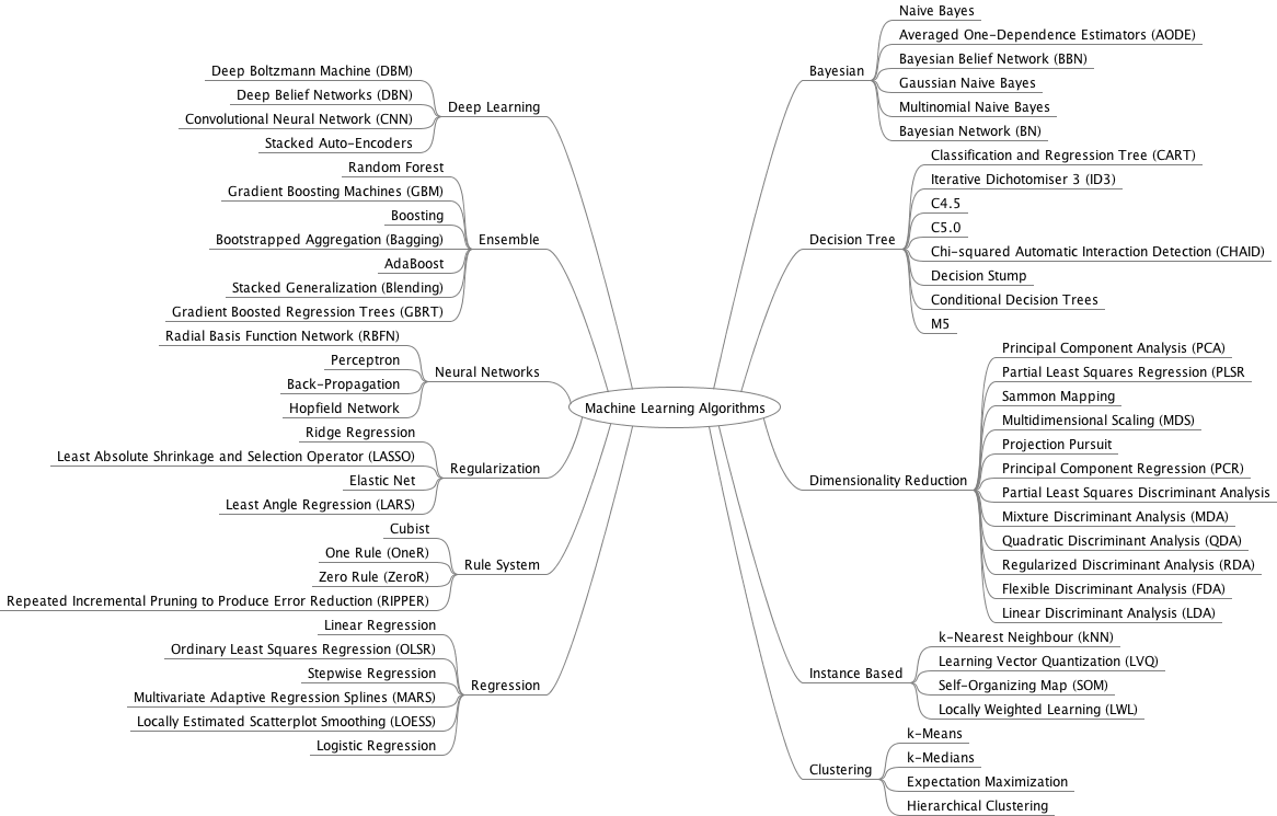

![Diversity of Machine Learning](MachineLearningAlgorithms.png)

---
name: Diversity of Machine Learning

## Supervised vs. Unsupervised

![Supervised vs. Unsupervised](SupervisedVsUnsupervisedAnalysis.png)

---
name: Supervised vs. Unsupervised

## Main Steps of Machine Learning

* To start Machine Learning one needs first to clean the data: impute, correct for batch-effects, normalize, standardize etc.

* Next step is to figure out features in the data. Note: Deep Learning skips this step and works directly on raw data

* Machine Learning model is fitted on the training and evaluated on an independent subset

![Main Steps of Machine Learning](ML.png)

---
name: Main Steps of Machine Learning

## How does Machine Learning work?

Machine Learning by default involves five basic steps:

1. Split data set into **train**, **validation** and **test** subsets.
2. Fit the model in the train subset.
3. Validate your model on the validation subset.
4. Repeat steps 1-3 a number of times and tune **hyperparameters**.
5. Test the accuracy of the optimized model on the test subset.

![Train-Test Split](TrainTestSplit.png)

---
name: How does Machine Learning work?

## Toy Example of Machine Learning

```r
set.seed(12345)
N<-100
x<-rnorm(N)
y<-2*x+rnorm(N)
df<-data.frame(x,y)
plot(y~x,data=df, col="blue")
```

---
name: Toy Example of Machine Learning

## Train and Test Subsets

We randomly assign 70% of the data to training and 30% to test subsets:

```r
set.seed(123)
train<-df[sample(1:dim(df)[1],0.7*dim(df)[1]),]
test<-df[!rownames(df)%in%rownames(train),]
```

---
name: Train and Test Subsets

## Validation of Model

```r
test_predicted<-as.numeric(predict(lm(y~x,data=train),newdata=test))
plot(test$y~test_predicted,ylab="True y",xlab="Pred y",col="darkgreen")
abline(lm(test$y~test_predicted),col="darkgreen")
```

---
name: Validation of Model

## Validation of Model (Cont.)

```r
summary(lm(test$y~test_predicted))
```

```
## 
## Call:
## lm(formula = test$y ~ test_predicted)
## 
## Residuals:
##     Min      1Q  Median      3Q     Max 
## -1.8383 -0.5789 -0.1077  0.5318  2.6054 
## 
## Coefficients:
##                Estimate Std. Error t value Pr(>|t|)    
## (Intercept)     0.05496    0.19107   0.288    0.776    
## test_predicted  0.92165    0.09442   9.762 1.64e-10 ***
## ---
## Signif. codes:  0 '***' 0.001 '**' 0.01 '*' 0.05 '.' 0.1 ' ' 1
## 
## Residual standard error: 1.03 on 28 degrees of freedom
## Multiple R-squared:  0.7729,	Adjusted R-squared:  0.7648 
## F-statistic: 95.29 on 1 and 28 DF,  p-value: 1.635e-10
```

Thus the model explains 76% of variation on the test subset.

---
name: Validation of Model (Cont.)

## What is a Hyperparameter?

* Hyperparameters are Machine Learning design parameters which are set before the learning process starts
* For the toy model a hyperparameter can be e.g. the number of covariates to adjust the main variable x of interest for

```r
set.seed(1)
for(i in 1:10)
{
  df[,paste0("PC",i)]<-1*(1-i/10)*y+rnorm(N)
}
head(df)
```

```
##            x          y color        PC1        PC2        PC3        PC4
## 1  0.5855288  1.3949830   red  0.6290309  0.4956198  1.3858900  1.7306635
## 2  0.7094660  0.2627087  blue  0.4200812  0.2522828  1.8727694 -0.8896729
## 3 -0.1093033  0.2038119  blue -0.6521979 -0.7478721  1.7292568  2.0936245
## 4 -0.4534972 -2.2317496  blue -0.4132938 -1.6273709 -1.8931325 -1.7226819
## 5  0.6058875  1.3528592  blue  1.5470811  0.4277027 -1.3382341  2.4658608
## 6 -1.8179560 -4.1719599  blue -4.5752323 -1.5702807 -0.4227104 -0.9909633
##          PC5         PC6         PC7        PC8        PC9       PC10
## 1  1.7719325  0.63529634  0.07742793 -0.4285716 -0.9474105 -1.5414026
## 2  2.0270091 -0.19178516  1.58123715  2.0241138 -1.7998121  0.1943211
## 3 -0.5010914 -1.10171748  0.58945128 -0.0492363  1.0156630  0.2644225
## 4 -1.5067426 -0.88140715 -0.12733353 -0.4603672 -0.2350367 -1.1187352
## 5  0.2602076  1.53274473  0.26918441 -0.8528851 -0.4643425  0.6509530
## 6 -2.4616374 -0.07481652 -2.38832183 -2.1785221 -0.5951440 -1.0329002
```

---
name: What is a Hyperparameter?

## How does Cross-Validation work?

* We should not include all PCs - overfitting
* Cross-Validation is a way to combat overfitting

```r
train<-df[sample(1:dim(df)[1],0.6*dim(df)[1]),]
val_test<-df[!rownames(df)%in%rownames(train),]
validate<-val_test[sample(1:dim(val_test)[1],0.25*dim(val_test)[1]),]
test<-val_test[!rownames(val_test)%in%rownames(validate),]
```
<img src="Presentation_MachineLearning_files/figure-html/unnamed-chunk-10-1.png" style="display: block; margin: auto auto auto 0;" />

---
name: How does Cross-Validation work?

## How does Cross-Validation work? (Cont.)

* Let us fit the linear regression model in the training set and validate the error in the validation data set
* Error: root mean squared difference between y predicted by the trained model for validation set and the real y in the validation set
* Looks like no drammatic decrease of RMSE after PC2

---
name: How does Cross-Validation work? (Cont.)

## Ultimate Model Evaluation

* Thus optimal model is y~x+PC1+PC2
* Perform final evaluation of the optimized/trained model on the test data set and report the final accuracy (adjusted R squared)
* The model explains over 90% of variation on the unseen test data set

```r
summary(lm(predict(lm(y~x+PC1+PC2,data=df),newdata=test)~test$y))
```

```
## 
## Call:
## lm(formula = predict(lm(y ~ x + PC1 + PC2, data = df), newdata = test) ~ 
##     test$y)
## 
## Residuals:
##     Min      1Q  Median      3Q     Max 
## -1.2789 -0.3681  0.0429  0.3976  0.9759 
## 
## Coefficients:
##             Estimate Std. Error t value Pr(>|t|)    
## (Intercept)  0.07429    0.11669   0.637     0.53    
## test$y       0.95907    0.04551  21.075   <2e-16 ***
## ---
## Signif. codes:  0 '***' 0.001 '**' 0.01 '*' 0.05 '.' 0.1 ' ' 1
## 
## Residual standard error: 0.5926 on 28 degrees of freedom
## Multiple R-squared:  0.9407,	Adjusted R-squared:  0.9386 
## F-statistic: 444.2 on 1 and 28 DF,  p-value: < 2.2e-16
```

---
name: Ultimate Model Evaluation

## What is Random Forest?

![Decision Tree](DecisionTree.png)

---
name: Random Forest

## Underfitting vs. Overfitting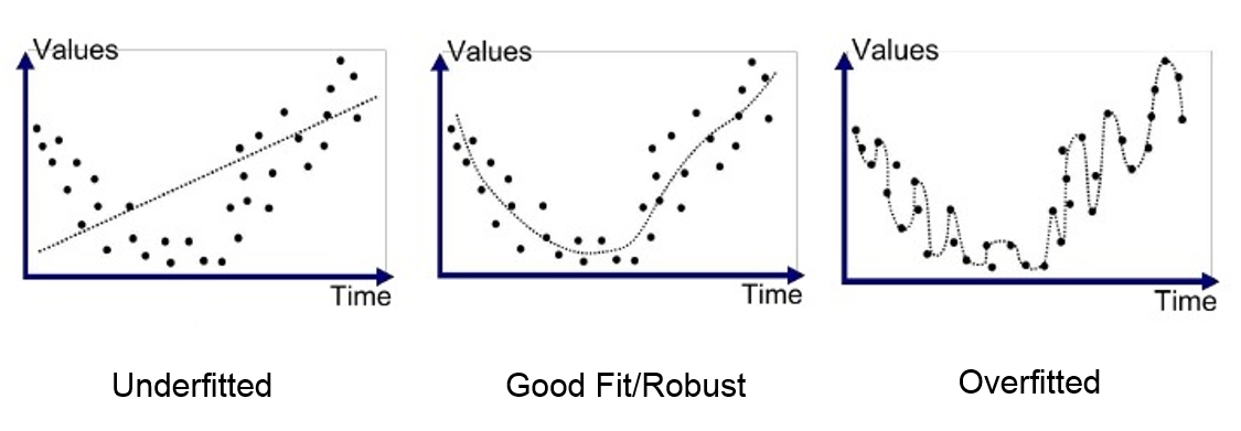

![Decision Tree](Underfitting_vs_Overfitting.png)

* Akaike Information Criterion (AIC):

`$$\rm AIC = 2k - 2ln(L)$$`
* Random Forest: each tree overfitted, but ensemble of trees performs very well

---
name: Underfitting vs. Overfitting

## Bias-Variance Tradeoff

.pull-left-50[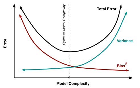
![Bias Variance](biasvariance.png)
]

.pull-right-50[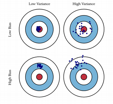
![Bias Variance Score](Bias_Variance_Score.png)
]

`$$Y = f(X) \Longrightarrow\rm{Reality} \\
Y = \hat{f}(X) + \rm{Error}\Longrightarrow\rm{Model} \\
Error^2 = (Y - \hat{f}(X))^2 = Bias^2 + Variance$$`

* It is mathematically proven that ensemble learning keeps the Bias the same but leads to a large decrease of Variance

---
name: Bias-Variance

## KNN and SVM

.pull-left-50[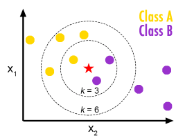
![kNN](kNN.png)

* How many out of K neighbors belong to each class

* Majority voting

* Non-linear

]
.pull-right-50[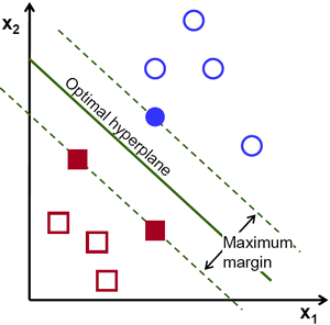
![SVM](SVM.png)

* Draw hyperplane that separates classes

* Maximize margins

* Can be linear and non-linear
]
---
name: KNN and SVM

## Classification: Pima Indians Diabetes

```r
library("mlbench")
data(PimaIndiansDiabetes2)
head(PimaIndiansDiabetes2,4)
```

```
##   pregnant glucose pressure triceps insulin mass pedigree age diabetes
## 1        6     148       72      35      NA 33.6    0.627  50      pos
## 2        1      85       66      29      NA 26.6    0.351  31      neg
## 3        8     183       64      NA      NA 23.3    0.672  32      pos
## 4        1      89       66      23      94 28.1    0.167  21      neg
```

```r
summary(results)
```

```
## 
## Call:
## summary.resamples(object = results)
## 
## Models: lda, cart, knn, svm, rf 
## Number of resamples: 50 
## 
## ROC 
##           Min.   1st Qu.    Median      Mean   3rd Qu.      Max. NA's
## lda  0.6774691 0.7923858 0.8356922 0.8268521 0.8730710 0.9398148    0
## cart 0.5642857 0.6827381 0.7323743 0.7351980 0.7822259 0.8796296    0
## knn  0.5516975 0.7515432 0.7836089 0.7817631 0.8286541 0.9452160    0
## svm  0.7079365 0.7808973 0.8287037 0.8238794 0.8688272 0.9285714    0
## rf   0.6753968 0.7800926 0.8040123 0.8119301 0.8497299 0.9483025    0
## 
## Sens 
##           Min.   1st Qu.    Median      Mean   3rd Qu.      Max. NA's
## lda  0.7222222 0.8392857 0.8734127 0.8811111 0.9166667 1.0000000    0
## cart 0.6388889 0.8055556 0.8611111 0.8585556 0.8888889 1.0000000    0
## knn  0.6944444 0.8055556 0.8611111 0.8547302 0.9079365 0.9444444    0
## svm  0.7222222 0.8333333 0.8611111 0.8642063 0.9160714 0.9722222    0
## rf   0.7222222 0.8113095 0.8611111 0.8592381 0.9166667 0.9722222    0
## 
## Spec 
##           Min.   1st Qu.    Median      Mean   3rd Qu.      Max. NA's
## lda  0.3333333 0.5000000 0.5555556 0.5531373 0.6111111 0.8888889    0
## cart 0.2222222 0.4444444 0.6111111 0.5637255 0.6666667 0.8333333    0
## knn  0.3333333 0.4199346 0.5000000 0.5062745 0.5555556 0.7777778    0
## svm  0.2222222 0.4444444 0.5000000 0.5211765 0.5972222 0.7777778    0
## rf   0.2941176 0.4444444 0.5000000 0.5260784 0.6111111 0.7777778    0
```

---
name: Classification: Pima Indians Diabetes

## Compare Machine Learning Methods

```r
dotplot(results)
```

---
name: Compare Machine Learning Methods

## Feature Selection

```r
feat<-varImp(best_model)$importance$pos
names(feat)<-rownames(varImp(best_model)$importance)
barplot(sort(feat,decreasing=T),ylab="FEATURE IMPORTANCE",col="darkred")
```

---
name: Feature Selection

## Make Predictions: Confusion Matrix

```r
predictions <- predict(best_model, test)
confusionMatrix(predictions, test$diabetes)
```

```
## Confusion Matrix and Statistics
## 
##           Reference
## Prediction neg pos
##        neg 131  42
##        pos  11  47
##                                           
##                Accuracy : 0.7706          
##                  95% CI : (0.7109, 0.8232)
##     No Information Rate : 0.6147          
##     P-Value [Acc > NIR] : 3.375e-07       
##                                           
##                   Kappa : 0.482           
##  Mcnemar's Test P-Value : 3.775e-05       
##                                           
##             Sensitivity : 0.9225          
##             Specificity : 0.5281          
##          Pos Pred Value : 0.7572          
##          Neg Pred Value : 0.8103          
##              Prevalence : 0.6147          
##          Detection Rate : 0.5671          
##    Detection Prevalence : 0.7489          
##       Balanced Accuracy : 0.7253          
##                                           
##        'Positive' Class : neg             
## 
```

---
name: Make Predictions

## ROC Curves on Test Data Set

---
name: ROC Curves

## What is Deep Learning?

* Artificial Neural Networks (ANN) with multiple layers

* Main advantages of Deep Learning over Machine Learning:
  * Feature extraction
  * Scalability

* Universal Approximation Theorem

---
name: What is Deep Learning?

## Artificial Neural Networks (ANN)

* Mathematical algorithm/function with special architecture

* Highly non-linear dues to activation functions

* Backward propagation for minimizing error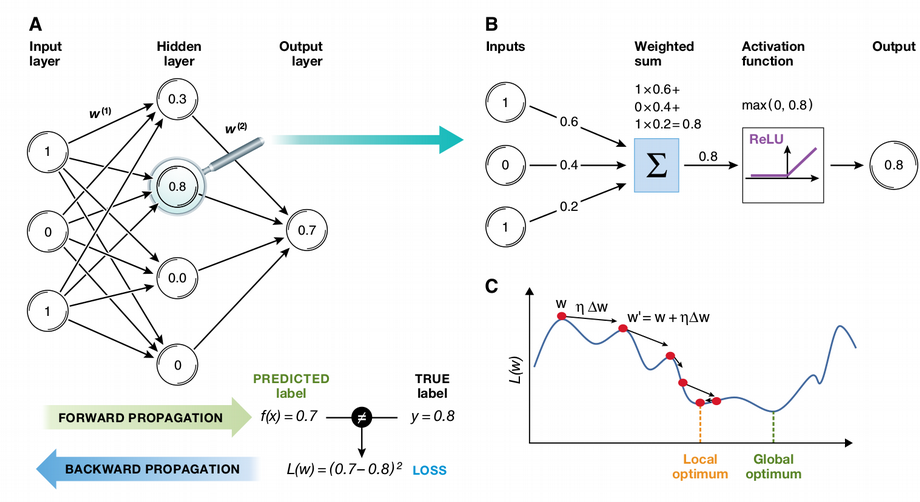

![ANN](ANN.png)

---
name: Artificial Neural Networks (ANN)

## Beauty of Neural Networks

* Maximum Likelihood
* Cross-Validation
* Bootstrapping
* Regularization
* Bayesian Inference
* Multivariate Feature Selection
* Monte Carlo Approximation
* Bagging and Boosting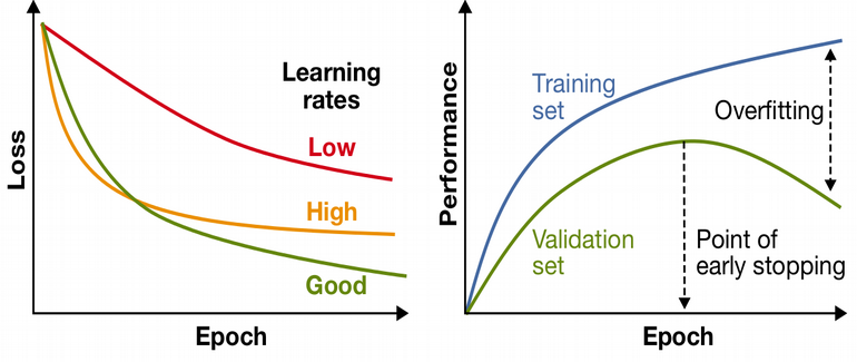

![Training](Training.png)

---
name: Beauty of Neural Networks

## Neural Network on Pima Indians

.pull-left-50[
<img src="Presentation_MachineLearning_files/figure-html/unnamed-chunk-24-1.png" style="display: block; margin: auto auto auto 0;" />
]

.pull-right-50[
<img src="CV_NumHidNeur.png" style="width: 100%;" />

```
## [1] "Confusion Matrix:"
##    
##       1   2
##   1 125  17
##   2  32  57
## [1] "Accuracy: 0.79"
```
]

---
name: Neural Network on Pima Diabetes Indians

---
name: end-slide
class: end-slide

# Thank you