Mathematical Statistics in R

class: center, middle, inverse, title-slide

# Mathematical Statistics in R
## Advanced R for Bioinformatics. Visby, 2018.
### Nikolay Oskolkov
### 15 Juni, 2018

---

class: spaced

## What is Mathematical Statistics?

* Can Mathematical Statistics mean
  * a statistical test? 
  * a probability distribution? 
  * or maybe a p-value?

* Classic statistics **is not the only way** to analyze your data

![Statistics](lies_and_statistics.png)

---
name: Statistics

## Different Types of Data Analysis

* Depends on the amount of data we have
* Balance between the numbers of features and observations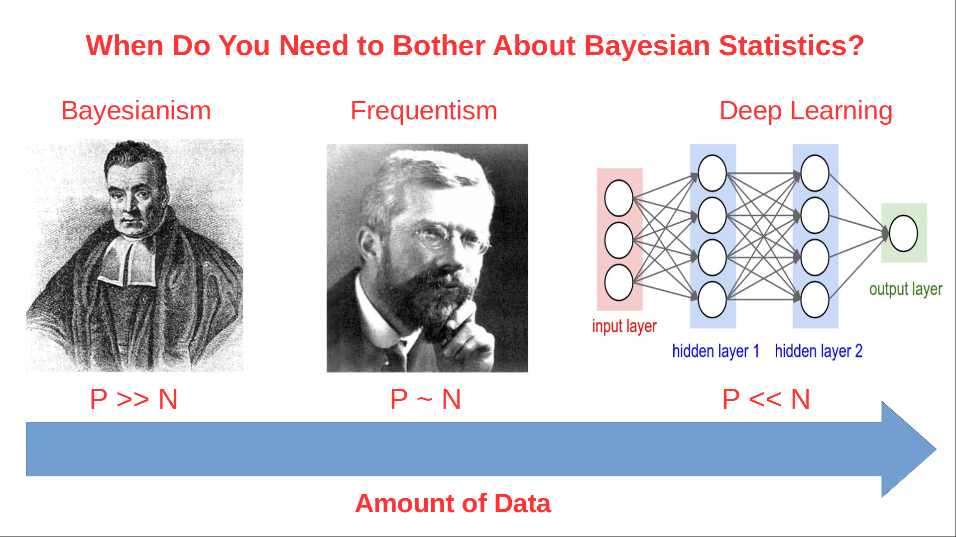

![Types of Analysis](AmountOfData.png)

---
name: Types of Analysis

## Frequentist Statistics Failure

![Anscombes quartet](Anscombes_quartet.png)

---
name: Frequentist Statistics Brain Damaging

## Frequentist Statistics Brain Damaging

![Data Saurus](DataSaurus.gif.png)

![Box Violin](BoxViolinSmaller.gif.png)

---
name: Frequentist Statistics Brain Damaging (Cont.)

## Maximum Likelihood Principle

* We maximize probability to observe the data `$X_i$`
`$$\rm{L}\,(\,\rm{X_i} \,|\, \mu,\sigma\,) =
\prod_{i=0}^{N}\frac{1}{\sqrt{2\pi\sigma²}} \exp^{\displaystyle -\frac{(X_i-\mu)^2}{2\sigma²}}\\
\mu = \frac{1}{N}\sum_{i=0}^N \rm{X_i}\\
\sigma^2 = \frac{1}{N}\sum_{i=0}^N (\rm{X_i}-\mu)^2$$`

* Maximum Likelihood has many assumptions:
  * Large sample size
  * Gaussian distribution
  * Homoscedasticity
  * Uncorrelated errors
  * Convergence of covariance
* Those assumptions are not fulfilled in the real world

---
name: Maximum Likelihood Principle

## Two-Groups Statistical Test

```r
set.seed(12)
X<-c(rnorm(20,mean=5,sd=2),12,15,14,16)
Y<-c(rnorm(24,mean=7,sd=2))
boxplot(X,Y,ylab="DIFFERENCE",names=c("X","Y"))
```

---
name: Statistical Test

## Parametric Statistical Test Fails

```r
t.test(X,Y)
```

```
## 
## 	Welch Two Sample t-test
## 
## data:  X and Y
## t = -1.084, df = 31.678, p-value = 0.2865
## alternative hypothesis: true difference in means is not equal to 0
## 95 percent confidence interval:
##  -2.8819545  0.8804344
## sample estimates:
## mean of x mean of y 
##  5.989652  6.990412
```
--
.center[
<img src="Presentation_GeneralStats_files/figure-html/unnamed-chunk-5-1.png" style="display: block; margin: auto auto auto 0;" />
]
---
name: Parametric Statistical Test

## Resampling

```r
observed <- median(Y)-median(X)
print(paste0("Observed difference = ",observed))
res <- vector(length=1000)
for(i in 1:1000){Z<-c(X,Y); Y_res<-sample(Z,length(Y),FALSE);
X_res<-sample(Z,length(X),FALSE); res[i]<-median(Y_res)-median(X_res)}
hist(abs(res), breaks=100, main="Resampled", xlab="Difference")
print(paste0("p-value = ", sum(abs(res) >= abs(observed))/1000))
```

```
## [1] "Observed difference = 2.33059085402647"
## [1] "p-value = 0.002"
```

<img src="Presentation_GeneralStats_files/figure-html/unnamed-chunk-6-1.png" style="display: block; margin: auto auto auto 0;" />
---
name: Resampling

## ML Does Not Stand Non-Independence

```
##            n1         n2         n3         n4          n5
## p1  1.0862296  0.2715666 -1.5000279 -2.1023121  0.47450044
## p2  0.5871922  1.1193045 -2.4755893 -0.7310311 -0.06784677
## p3  1.8750843  1.2789147  0.4295881  0.8118376 -0.22511970
## p4  0.4396084 -0.1569604 -0.3682398  0.8253523  0.23070668
## p5 -0.4962881 -1.0323406 -0.9390560 -0.4715313  0.35579237
```

* Two types of non-independence in data
  * between samples
  * between features

.pull-left-50[
### Random Effects
<img src="Random_Effects.jpg" style="width: 60%;" />]
.pull-right-50[
### Lasso
<img src="lasso.jpg" style="width: 40%;" />]

---
name: ML Does Not Stand Non-Independence

## Linear Model with Non-Independence

```r
library("lme4")
library("ggplot2")
ggplot(sleepstudy,aes(x=Days,y=Reaction)) + geom_point() + 
  geom_smooth(method="lm")
```

<img src="Presentation_GeneralStats_files/figure-html/unnamed-chunk-8-1.png" style="display: block; margin: auto auto auto 0;" />
---
name: Linear Model with Non-Independence

## Fit Linear Model for Each Individual

```r
ggplot(sleepstudy, aes(x = Days, y = Reaction)) + 
  geom_smooth(method = "lm", level = 0.95) + geom_point() + 
  facet_wrap( ~ Subject, nrow = 3, ncol = 6)
```

<img src="Presentation_GeneralStats_files/figure-html/unnamed-chunk-9-1.png" style="display: block; margin: auto auto auto 0;" />
---
name: Fit Linear Model for Each Individual

## Random Effects and Missing Heritability

---
name: The Case of the Missing Heritability

## Random Effects Modelling

* Allow individual level Slopes and Intercepts
* This is nothing else than Bayesian Priors on coefficients

`$$\rm{Reaction} = \alpha_i + \beta_i \rm{Days}$$`

```r
lmerfit <- lmer(Reaction ~ Days + (Days | Subject), sleepstudy)
```
.pull-left-50[
<img src="Presentation_GeneralStats_files/figure-html/unnamed-chunk-11-1.png" style="display: block; margin: auto auto auto 0;" />
]
.pull-right-50[
<img src="Presentation_GeneralStats_files/figure-html/unnamed-chunk-12-1.png" style="display: block; margin: auto auto auto 0;" />
]

---
name: Random Effects Modelling

## Linear Mixed Models (LMM)

```r
summary(lmer(Reaction ~ Days + (Days | Subject), sleepstudy))
```

```
## Linear mixed model fit by REML ['lmerMod']
## Formula: Reaction ~ Days + (Days | Subject)
##    Data: sleepstudy
## 
## REML criterion at convergence: 1743.6
## 
## Scaled residuals: 
##     Min      1Q  Median      3Q     Max 
## -3.9536 -0.4634  0.0231  0.4634  5.1793 
## 
## Random effects:
##  Groups   Name        Variance Std.Dev. Corr
##  Subject  (Intercept) 612.09   24.740       
##           Days         35.07    5.922   0.07
##  Residual             654.94   25.592       
## Number of obs: 180, groups:  Subject, 18
## 
## Fixed effects:
##             Estimate Std. Error t value
## (Intercept)  251.405      6.825  36.838
## Days          10.467      1.546   6.771
## 
## Correlation of Fixed Effects:
##      (Intr)
## Days -0.138
```
---
name: Linear Mixed Models (LMM)

## LMM Average Fit

---
name: LMM Average Fit

## LMM Individual Fit

---
name: LMM Individual Fit

## What is Bayesian Statistics for You?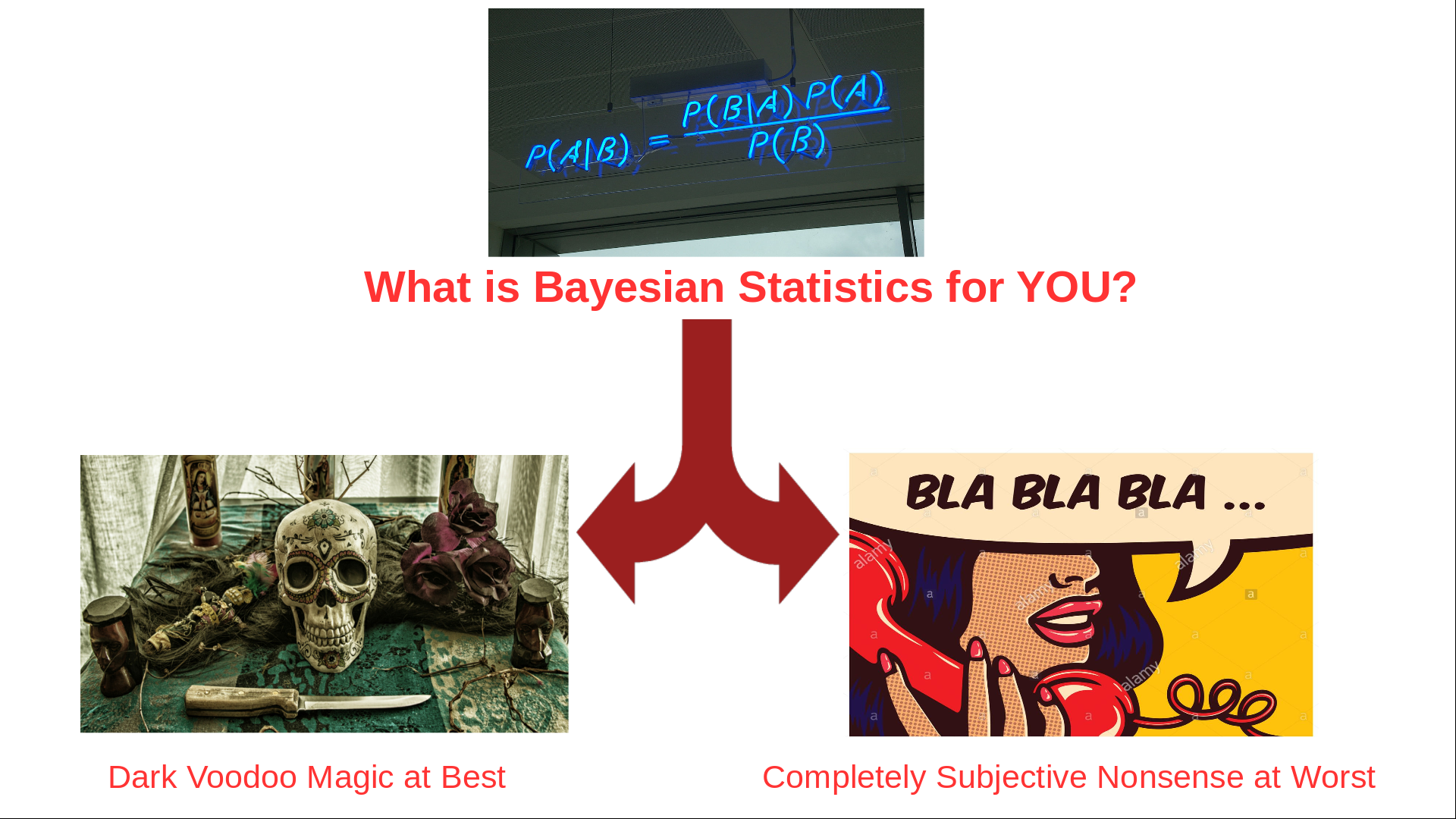

![What is Bayesian Statistics for You?](BayesianStatistics.png)

.small[
* **Handling Missing Data**
* **Handling Non-Gaussian Data**
* **Cause or Consequence**
* **Lack of Statistical Power**
* **Overfitting and Correction for Multiple Testing (FDR)**
* **Testing for Significance and P-Value**
]

---
name: What is Bayesian Statistics for You?

## Frequentist vs. Bayesian Linear Model

.pull-left-50[
### Maximum Likelihood
`$$y = \alpha+\beta x$$`
`$$L(y) \sim e^{-\frac{(y-\alpha-\beta x)^2}{2\sigma^2}}$$`
`$$\max_{\alpha,\beta,\sigma}L(y) \Longrightarrow \hat\alpha, \hat\beta, \hat\sigma$$`
]
--
.pull-right-50[
### Bayesian Linear Fitting
`$$y \sim \it N(\mu,\sigma) \quad\rightarrow \textrm{Likelihood}:L(y| \mu,\sigma)$$`
`$$\mu = \alpha + \beta x \quad \textrm{(deterministic)}$$`
`$$\alpha \sim \it N(\mu_\alpha,\sigma_\alpha) \quad\rightarrow\textrm{Prior on} \quad\alpha:P(\alpha|\mu_\alpha,\sigma_\alpha)$$`
`$$\beta \sim \it N(\mu_\beta,\sigma_\beta) \quad\rightarrow\textrm{Prior on} \quad\beta: P(\beta|\mu_\beta,\sigma_\beta)$$`
`$$P(\alpha, \beta|y, \mu_\alpha,\sigma_\alpha,\mu_\beta,\sigma_\beta, \sigma) =  \frac{L(y|\mu,\sigma) P(\alpha|\mu_\alpha,\sigma_\alpha)P(\beta|\mu_\beta,\sigma_\beta)}{\int_{\alpha,\beta,\sigma}L(y|\mu,\sigma) P(\alpha|\mu_\alpha,\sigma_\alpha)P(\beta|\mu_\beta,\sigma_\beta)}$$`
`$$\max_{\alpha,\beta,\sigma}P(\alpha, \beta, \sigma|y, \mu_\alpha,\sigma_\alpha,\mu_\beta,\sigma_\beta) \Longrightarrow \hat\alpha,\hat\beta,\hat\sigma$$`

]

---
name: Frequentist vs. Bayesian Fitting

## Bayesian Linear Model

```r
library("brms")
options(mc.cores = parallel::detectCores())
brmfit <- brm(Reaction ~ Days + (Days | Subject), data = sleepstudy)
summary(brmfit)
```

```
##  Family: gaussian 
##   Links: mu = identity; sigma = identity 
## Formula: Reaction ~ Days + (Days | Subject) 
##    Data: sleepstudy (Number of observations: 180) 
## Samples: 4 chains, each with iter = 2000; warmup = 1000; thin = 1; 
##          total post-warmup samples = 4000
##     ICs: LOO = NA; WAIC = NA; R2 = NA
##  
## Group-Level Effects: 
## ~Subject (Number of levels: 18) 
##                     Estimate Est.Error l-95% CI u-95% CI Eff.Sample Rhat
## sd(Intercept)          26.99      6.84    15.68    42.52       1869 1.00
## sd(Days)                6.61      1.53     4.19    10.12       1591 1.00
## cor(Intercept,Days)     0.09      0.30    -0.48     0.68        978 1.00
## 
## Population-Level Effects: 
##           Estimate Est.Error l-95% CI u-95% CI Eff.Sample Rhat
## Intercept   251.22      7.23   236.75   265.84       1592 1.00
## Days         10.47      1.72     7.13    13.89       1332 1.00
## 
## Family Specific Parameters: 
##       Estimate Est.Error l-95% CI u-95% CI Eff.Sample Rhat
## sigma    25.85      1.55    23.08    29.17       4000 1.00
## 
## Samples were drawn using sampling(NUTS). For each parameter, Eff.Sample 
## is a crude measure of effective sample size, and Rhat is the potential 
## scale reduction factor on split chains (at convergence, Rhat = 1).
```
---
name: Bayesian Linear Model

## Bayesian Population-Level Fit

---
name: Bayesian Population-Level Fit

## Bayesian Group-Level Fit

---
name: Bayesian Group-Level Fit

## Feature Non-Independence: LASSO

`$$Y = \beta_1X_1+\beta_2X_2+\epsilon \\
\textrm{OLS} = (y-\beta_1X_1-\beta_2X_2)^2 \\
\textrm{Penalized OLS} = (y-\beta_1X_1-\beta_2X_2)^2 + \lambda(|\beta_1|+|\beta_2|)$$`

.center[
<img src="CV_lambda.png" style="width: 60%;" />]

---
name: Feature Non-Independence: LASSO

## Dimensionality Reduction

* Can Dimensionality Reduction mean
  * PCA? 
  * tSNE?

.pull-left-50[
.pull-right-50[
<img src="PCA.png" style="width: 100%;" />]]
.pull-right-50[
<img src="tSNE.png" style="width: 50%;" />]

--
.pull-left-50[
.pull-right-50[
<img src="DarkMagic.jpg" style="width: 100%;" />]]
.pull-right-50[
No, this is about overcoming

**The Curse of Dimenionality**

also known as Rao's Paradox
]

---
name: Dimensionality Reduction

## Low Dimensional Space

```r
set.seed(123); n <- 20; p <- 2
Y <- rnorm(n); X <- matrix(rnorm(n*p),n,p); summary(lm(Y~X))
```

```
## 
## Call:
## lm(formula = Y ~ X)
## 
## Residuals:
##     Min      1Q  Median      3Q     Max 
## -2.0522 -0.6380  0.1451  0.3911  1.8829 
## 
## Coefficients:
##             Estimate Std. Error t value Pr(>|t|)
## (Intercept)  0.14950    0.22949   0.651    0.523
## X1          -0.09405    0.28245  -0.333    0.743
## X2          -0.11919    0.24486  -0.487    0.633
## 
## Residual standard error: 1.017 on 17 degrees of freedom
## Multiple R-squared:  0.02204,	Adjusted R-squared:  -0.09301 
## F-statistic: 0.1916 on 2 and 17 DF,  p-value: 0.8274
```
---
name: Low Dimensional Space

## Going to Higher Dimensions

```r
set.seed(123456); n <- 20; p <- 10
Y <- rnorm(n); X <- matrix(rnorm(n*p),n,p); summary(lm(Y~X))
```

```
## 
## Call:
## lm(formula = Y ~ X)
## 
## Residuals:
##     Min      1Q  Median      3Q     Max 
## -1.0255 -0.4320  0.1056  0.4493  1.0617 
## 
## Coefficients:
##             Estimate Std. Error t value Pr(>|t|)  
## (Intercept)  0.54916    0.26472   2.075   0.0679 .
## X1           0.30013    0.21690   1.384   0.1998  
## X2           0.68053    0.27693   2.457   0.0363 *
## X3          -0.10675    0.26010  -0.410   0.6911  
## X4          -0.21367    0.33690  -0.634   0.5417  
## X5          -0.19123    0.31881  -0.600   0.5634  
## X6           0.81074    0.25221   3.214   0.0106 *
## X7           0.09634    0.24143   0.399   0.6992  
## X8          -0.29864    0.19004  -1.571   0.1505  
## X9          -0.78175    0.35408  -2.208   0.0546 .
## X10          0.83736    0.36936   2.267   0.0496 *
## ---
## Signif. codes:  0 '***' 0.001 '**' 0.01 '*' 0.05 '.' 0.1 ' ' 1
## 
## Residual standard error: 0.8692 on 9 degrees of freedom
## Multiple R-squared:  0.6592,	Adjusted R-squared:  0.2805 
## F-statistic: 1.741 on 10 and 9 DF,  p-value: 0.2089
```
---
name: Going to Higher Dimensions

## Even Higher Dimensions

```r
set.seed(123456); n <- 20; p <- 20
Y <- rnorm(n); X <- matrix(rnorm(n*p),n,p); summary(lm(Y~X))
```

```
## 
## Call:
## lm(formula = Y ~ X)
## 
## Residuals:
## ALL 20 residuals are 0: no residual degrees of freedom!
## 
## Coefficients: (1 not defined because of singularities)
##             Estimate Std. Error t value Pr(>|t|)
## (Intercept)  1.34889         NA      NA       NA
## X1           0.66218         NA      NA       NA
## X2           0.76212         NA      NA       NA
## X3          -1.35033         NA      NA       NA
## X4          -0.57487         NA      NA       NA
## X5           0.02142         NA      NA       NA
## X6           0.40290         NA      NA       NA
## X7           0.03313         NA      NA       NA
## X8          -0.31983         NA      NA       NA
## X9          -0.92833         NA      NA       NA
## X10          0.18091         NA      NA       NA
## X11         -1.37618         NA      NA       NA
## X12          2.11438         NA      NA       NA
## X13         -1.75103         NA      NA       NA
## X14         -1.55073         NA      NA       NA
## X15          0.01112         NA      NA       NA
## X16         -0.50943         NA      NA       NA
## X17         -0.47576         NA      NA       NA
## X18          0.31793         NA      NA       NA
## X19          1.43615         NA      NA       NA
## X20               NA         NA      NA       NA
## 
## Residual standard error: NaN on 0 degrees of freedom
## Multiple R-squared:      1,	Adjusted R-squared:    NaN 
## F-statistic:   NaN on 19 and 0 DF,  p-value: NA
```
---
name: Even Higher Dimensions

## The Math Blows Up in High Dimensions

Let us now take a closer look at why exactly the ML math blows up when n<=p. Consider a linear model:

`$$Y = \beta X$$`

Let us make a few mathematical tricks in order to get a solution for the coefficients of the linear model:

`$$X^TY = \beta X^TX \\
(X^TX)^{-1}X^TY = \beta(X^TX)^{-1} X^TX \\
(X^TX)^{-1}X^TY = \beta$$`

The inverse matrix `$(X^TX)^{-1}$` **diverges** when p=>n as variables in X become correlated

---
name: Maximum Likelihood Blows Up

## No True Effects in High Dimensions

.pull-left-50[

```r
set.seed(12345)
N <- 100
x <- rnorm(N)
y <- 2*x+rnorm(N)
df <- data.frame(x,y)
```
]
.pull-right-50[

```r
for(i in 1:10)
{
df[,paste0("PC",i)]<-
  Covar*(1-i/10)*y+rnorm(N)
}
```
]
.center[
<img src="Presentation_GeneralStats_files/figure-html/unnamed-chunk-24-1.png" style="display: block; margin: auto auto auto 0;" />
]
---
name: No True Effects in High Dimensions

## Principal Component Analysis (PCA)

* Collapse p features (p>>n) to few latent features and keep variation

* Rotation and shift of coordinate system toward maximal variance

* PCA is an **eigen matrix decomposition** problem

.pull-left-50[
<img src="pca_demo.gif" style="width: 100%;" />]
.pull-right-50[
`$$PC = u^T X = X^Tu$$`
X is mean centered `$\Longrightarrow <PC> = 0$`
`$$<(PC-<PC>)^2> = <PC^2> = u^T X X^Tu \\
X X^T=A \\ 
< PC^2 > = u^T Au$$`
A is **variance-covariance** of X

`$$\rm{max}(u^T Au + \lambda(1-u^Tu))=0 \\
 Au = \lambda u$$`
]
---
name: PCA

## PCA on MNIST

---
name: PCA on MNIST

## t-distributed Stochastic Neighbor Embedding (tSNE)

.center[
<img src="tSNE_Scheme.png" style="width: 65%;" />]

---
name: tSNE

## tSNE on MNIST

---
name: tSNE on MNIST

---
name: end-slide
class: end-slide

# Thank you